Highlight: Hello and welcome to the sixth part of our OpenCV with Python post series. In this post we will cover some basic image arithmetic. You will learn how to perform some elementary arithmetic operations on images like addition and subtraction. In addition we will talk about logical bitwise operations (AND, OR, XOR, NOT). Also, we will see how we can implement these operations in some practical tasks in Python. For example, we will explain how to combine them and how to blend several images to get spectacular Photoshop-like effects. So, let’s start.

Tutorial Overview:

1. Image addition and subtraction
2. Logical bitwise operations on images (AND, OR, XOR, NOT)

1. Image addition and subtraction

We are all familiar with adding, subtracting or multiplying two numbers. That easy, right? Well, it may be easy when we are operating with numbers, but things are a little bit trickier when we start working with images. The reason for that is that images have limits in both color space and data type, so addition and subtraction cannot be applied in a common way.

So, let’s imagine two pixels in a two different images and we want to add them. How can we add them? In order to do that, let’s imagine the folowing scenario. The first pixel has a color intensity of (200, 0, 0) and the second one has color intensity of (100, 0, 0). If we simply add these values together our result will be (300, 0, 0). However, this is not possible when we are dealing with RGB images because they are represented as 8-bit unsigned integers (0, 255). So, how can we solve this problem in Python? The solution comes with OpenCV library that has implemented cv2.add() and cv2.subtract() functions.

First, we will start our code snippet with a simple addition.

# Necessary imports
import numpy as np
import cv2
import matplotlib.pyplot as plt
from google.colab.patches import cv2_imshow

#  Creating 8-bit array of one element 200
x = np.uint8([200])
#  Creating 8-bit array of one element 100
y = np.uint8([100])
# Adding our arrays
result = x + y
print("x:'{}' + y:'{}' = '{}'".format(x, y, result))

Numpy Output: x:'[200]’ + y:'[100]’ = ‘[44]’

As you can see our result is 44. Maybe you haven’t expected this. So, what happened? Well, we got an overflow. Such a result is obtained because in NumPy, the values are wrapped around. To visualize this, you can imagine a big digital stopwatch where instead of 60 we have 255. After reaching a maximum value of 255 the next number can’t be registered. So, instead of 256 our next number will be 0. This is also called a modulo operation.

To overcome this challenge with “uint” type that we have to use with images, OpenCV has an implemented functioncv2.add(). Contrary to the previous case, OpenCV makes sure that when overflow happens, we will register maximum element which is 255. This is also called a saturated operation.

#  Creating 8-bit array of one element 200
x = np.uint8([200])
#  Creating 8-bit array of one element 100
y = np.uint8([100])
# Adding our arrays with cv2.add()
result=cv2.add(x,y)
print("x:'{}' + y:'{}' = '{}'".format(x, y, result))

CV Output: x:'[200]’ + y:'[100]’ = ‘[[255]]’

We can see that addition with cv2.add() function returned a maximum value of 255. Now, let’s have a look at similar example with subtraction. For that operation we are going to use function cv2.subtract().

#  Creating 8-bit array of one element 200
x = np.uint8([200])
#  Creating 8-bit array of one element 100
y = np.uint8([100])
# Sbtracting our arrays
result = y - x
print("y:'{}' - x:'{}' = '{}'".format(y, x, result))

Numpy Output: y:'[100]’ – x:'[200]’ = ‘[156]’

#  Creating 8-bit array of one element 200
x = np.uint8([200])
#  Creating 8-bit array of one element 100
y = np.uint8([100])
# Sbtracting our arrays
result =cv2.subtract(y, x) 
print("y:'{}' - x:'{}' = '{}'".format(y, x, result))

CV Output: y:'[100]’ – x:'[200]’ = ‘[[0]]’

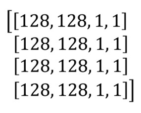
In order to understand how addition and subtraction works we will use our mini toy image. This image will consist of only 16 pixels \(( 4\times 4 ) \).

# Creating the first 4 x 4 image with values of 1s
A = np.ones( (4,4), dtype = 'uint8')
# Changing our values from column 0 to column 2
A[:,0:2] = 128 
print(A)

Output:

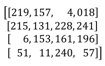
# The second image of size 4 x 4 is created using randint function
# Creating the second 4 x 4 image with random integer values
B= np.random.randint(0,255,4*4, dtype = 'uint8')
B = B.reshape(  (4,4) )
print(B)

Output:

# Adding two images with cv2.add() function
C_sum_cv2 = cv2.add(A, B)
# Adding two images in Numpy
C_sum  = A + B
print(C_sum_cv2)
print(C_sum)

# Subtracting two images with cv2.subtract() function
C_sub_cv2 = cv2.subtract(B, A)
print(C_sub_cv2)
# Subtracting two images in Numpy
C_sub = B - A
print(C_sub)

Output:

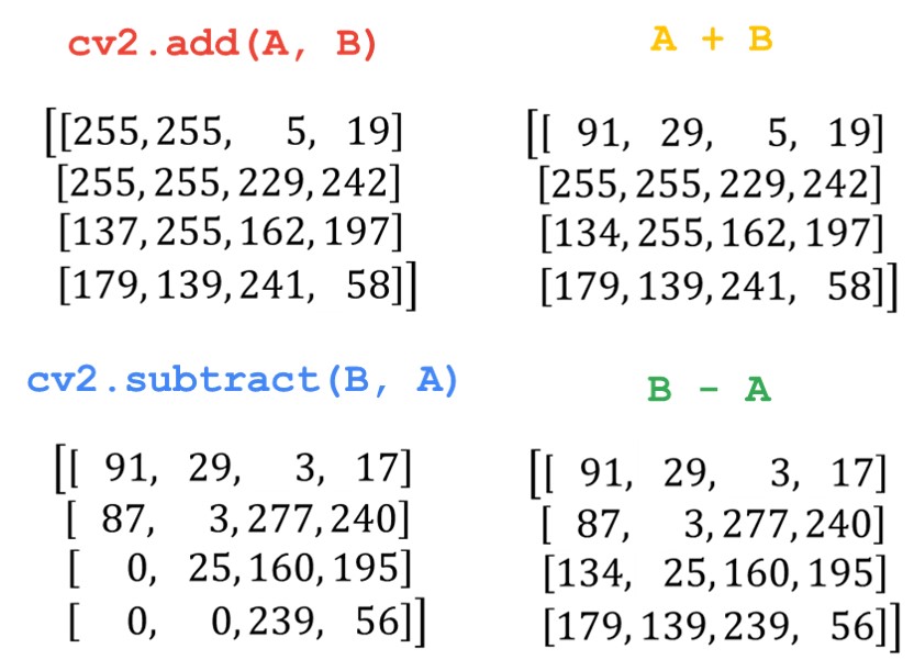
Image saturation

Operations like addition and subtraction can help us to make images brighter or darker. One way to do this is to create duplicate for our original image with identical pixel values. In other words, we will do this by creating an image that has identical dimensions as our original image with all pixel values 1. Then, we will multiply this image with the appropriate scalar (in our case that is a value 100). In that way we have obtained a gray image. When we add this gray image to the original one, our original image will become brighter. As the resulting images are closer to 255 our image will become brighter. On the other hand, if we subtract the gray image from the original one, the pixel values will decrease and our original image will become darker. If the result of subtracted pixel values is 0, our pixels will become black.

# Loading the image
img = cv2.imread('GoT.jpg',1)
cv2_imshow(img)

Output:

# Creating an image of 1s with the same size 
# as our input image
img_100 = np.ones(img.shape, dtype = "uint8") * 100
# Adding two images
img2=cv2.add(img,img_100)
cv2_imshow(img2)

# Subtracting two images
img3=cv2.subtract(img,img_100)
cv2_imshow(img3)

Output:

Image blending

If we want to blend two images together we need use a function called cv2.addWeighted(). We can use this method when we want to give different weights to our images which will give us an impression of transparency. So, for example, if we want to add 90% of our first image to 10% of our second image we will use this function. There are several parameters that we are going to use in this method as you can see in the following example.

Now, let’s add dataHacker logo to our image. We need images of a same size so the first thing that we are going to do is to create an image with identical dimensions as our original image with all pixel values of 1. Then, we will define a central area of our black image and add the image of a logo to it.

# Loading our logo
logo = cv2.imread("Datahacker_logo.jfif",1) 
cv2_imshow(logo)

Output:

 # Creating an image of 1s with the same size 
 # as our input image
 img_1 = np.ones(img.shape, dtype = "uint8") 

(wl, hl) = (logo.shape[1] ,logo.shape[0] )
(w,h)=(img_1.shape[1], img_1.shape[0])
img_1[(h//2 - hl//2)+50 : (h//2 + hl//2)+50, (w//2-wl//2) : (w//2 + wl//2),:]=logo
cv2_imshow(img_1)

Output:

# Blending our two images
img_blend=cv2.addWeighted(img, 0.6, img_1, 0.4, 0)
cv2_imshow(img_blend)

Output:

It is good to remember that function cv2.addWeighted() is commonly used to combine the outputs of the Sobel operator.

2. Logical bitwise operations on images (AND, OR, XOR, NOT)

You may wonder why we actually use the bitwise operations. Well, their origin dates from old computer monitors when we had only two values: 0 and 1 or black and white.

And guess what. Once we have binary image on this screen we can play around with logical bitwise operations. They are very important logical operations and we use them when we want to manipulate the values of the image for comparisons and calculations. There are four of these operations and they are very simple, and easy to understand.

• AND – True if both pixels are greater than zero
• OR – True if either of the two pixels are greater than zero
• XOR – True if either of the two pixels are greater than zero, but not both
• NOT – Invert pixel values

Bitwise operations are applied on grayscale images. First of all, they convert a grayscale into a binary images as you can see in a following example. The rule for conversion is the folowing: any given pixel larger then zero will become one, and zeros will remain zeros. In another words, any given pixel with value “0” is represented with number zero (pixel is turned “off”), and any pixel with value greater than “0” is represented with number one (pixel is turned “on”).  

Now lets apply bitwise operations on our binary images.

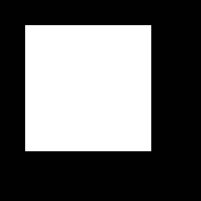
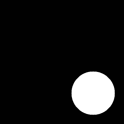
In order to better explain how these operations work, we will create two images. In the first one we will draw a rectangle and in the second one we will draw a circle. Then, we will apply bitwise operations on them and observe what we will get as output.

# Creating an image with 1s and drawing white rectangle on it
img_rectangle = np.ones((400,400), dtype = "uint8") 
cv2.rectangle(img_rectangle, (50,50), (300,300), (255,255,255), -1)
cv2_imshow(img_rectangle)

Output:

.

# Creating an image with 1s and drawing white circle on it
img_circle = np.ones((400,400), dtype = "uint8") 
cv2.circle(img_circle, (300,300), 70, (255,255,255), -1)
cv2_imshow(img_circle)

Output:

# Applying a bitwise AND to our rectangle and circle
bitwiseAnd = cv2.bitwise_and(img_rectangle,img_circle)
cv2_imshow(bitwiseAnd)
# Applying a bitwise OR to our rectangle and circle
bitwiseOr = cv2.bitwise_or(img_rectangle,img_circle)
cv2_imshow(bitwiseOr)
# Applying a bitwise XOR to our rectangle and circle
bitwiseXor = cv2.bitwise_xor(img_rectangle,img_circle)
cv2_imshow(bitwiseXor)
# Applying a bitwise NOT to our rectangle 
bitwiseNot_rec = cv2.bitwise_not(img_rectangle)
cv2_imshow(bitwiseNot_rec)
# Applying a bitwise NOT to our circle 
bitwiseNot_circ = cv2.bitwise_not(img_circle)
cv2_imshow(bitwiseNot_circ)

Output:

Masking

A extremely useful technique in the image processing is masking, which allows us to focus only on the special part or area of the image.

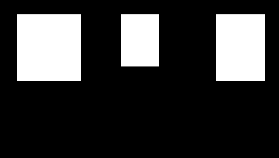
So, let’s assume that we want to highlight parts of the image with faces on it and ignore the rest of the image. First, we need to construct our mask. To do that we will create a NumPy array of zeros, with the same size as our original image. Then, we will draw 3 white rectangles on it. The Coordinates of those rectangles will correspond to the position of three faces in our image. And finally, we can apply cv2.bitwise_and() function in order to obtain our output. The function will be True if both pixels are greater than zero and in our case those pixels are inside the white rectangle.

# Creating an image of 1s with the same size 
# as our input image
mask = np.zeros(img.shape, dtype = "uint8")
# Drawing rectangle that corresponds to the first face
# on the image
cv2.rectangle(mask, (60,50), (280,280), (255,255,255), -1)
# Drawing rectangle that corresponds to the second face
# on the image
cv2.rectangle(mask, (420,50), (550,230), (255,255,255), -1)
# Drawing rectangle that corresponds to the third face
# on the image
cv2.rectangle(mask, (750,50), (920,280), (255,255,255), -1)
cv2_imshow(mask)

Output:

# Applying a bitwise AND to the mask and image
masked = cv2.bitwise_and(img,mask)
cv2_imshow(masked)

Output:

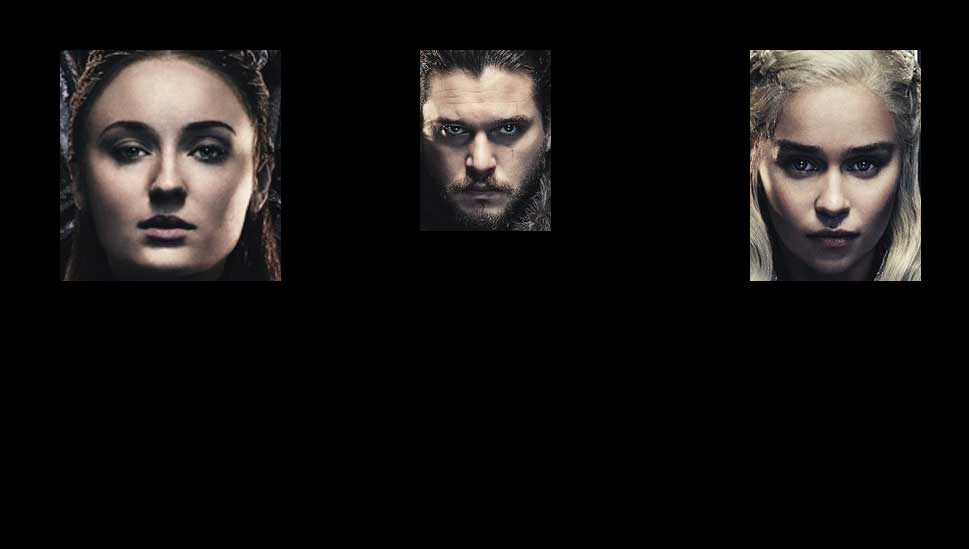
As you can see using bitwise operations, we can focus only on regions of the image that interests us. This technique will be particularly useful in the future when we start to learn how to perform some image recognition task.

Summary

In this post, we reviewed basic arithmetic operations that we can apply on images. We learn how to add and subtract two images, how to blend them and to apply effects like saturation. Also, we explained what bitwise operation are and why they are extremely important for our future image processing tasks.

References:

[1] Mastering OpenCV 4 with Python by Alberto Fernández Villán

[2] Practical Python and OpenCV by Adrian Rosebrock