#011 TF YOLO V3 Object Detection in TensorFlow 2.0
YOU ONLY LOOK ONCE
Highlights: Prior to Yolo majority of approaches for object detection tried to adapt the classifiers for the purpose of detection. In YOLO, an object detection has been framed as a regression problem to spatially separated bounding boxes and associated class probabilities. In this post we will learn about the YOLO Object Detection system, and how to implement such a system in TensorFlow 2.0.

About Yolo:
— You Only Look Once: Unified, Real-Time Object Detection, 2015
Our unified architecture is extremely fast. Our base YOLO model processes images
in real-time at 45 frames per second. A smaller version of the network, Fast YOLO,
processes an astounding 155 frames per second …
Tutorial Overview:
1. What is Yolo?
Yolo is a state-of-the-art, object detection system (network). It was developed by Joseph Redmon. The biggest advantage over other popular architectures is speed. The Yolo model family models are really fast, much faster than R-CNN and others. This means that we can achieve real-time object detection.
At the time of first publishing (2016.) compared to systems like R-CNN and DPM, YOLO has achieved the state-of-the-art mAP (mean Average Precision). On the other hand, YOLO struggles to accurately localize objects. However, it learns general representation of the objects. In newer version, there are some improvements in both speed and accuracy.
Alternatives (at the time of the publishing): Other approaches mainly used a sliding window approach over the entire image and the classifier is used on these regions (DPM – deformable part models). In addition, R-CNN used region proposal method. This method first generated potential bounding boxes. Then, a classifier was run on those boxes, and post-processing has been applied to remove duplicate detections and refine bounding boxes.
YOLO has reframed an object detection problem into a single regression problem. It goes directly from image pixels, up to bounding box coordinates and class probabilities. Hence, a single convolutional network predicts multiple bounding boxes and class probabilities for those boxes.
2. Theory
As Yolo works with only one look at the image, sliding windows is not the right approach. Instead, the entire image can be splitted into the grid. This grid will be \(S \times S\) dimensions. Now, each cell is responsible for predicting a few different things.
First thing, each cell is responsible for predicting some number of bounding boxes. Also, each cell will predict confidence value for each bounding box. In other word, this is a probability that a box contains an object. In case that there is no object in some grid cell, it is important that confidence value is very low for that cell.
When we visualize all of these predictions, we get a map of all the objects and a bunch of boxes which is ranked by their confidence value.

The second thing, each cell is responsible for predicting class probabilities. This is not saying that some grid cell contains some object, this is just a probability. So, if a grid cell predicts car, it is not saying that there is a car, it is just saying that if there is an object, than that object is a car.
Let us describe in more details how output looks like.
In Yolo, anchor boxes are used to predict bounding boxes. The main idea of anchor boxes is to predefine two different shapes. They are called anchor boxes or anchor box shapes. In this way, we will be able to associate two predictions with the two anchor boxes. In general, we might use even more anchor boxes (five or even more). Anchors were calculated on the COCO dataset using k-means clustering.
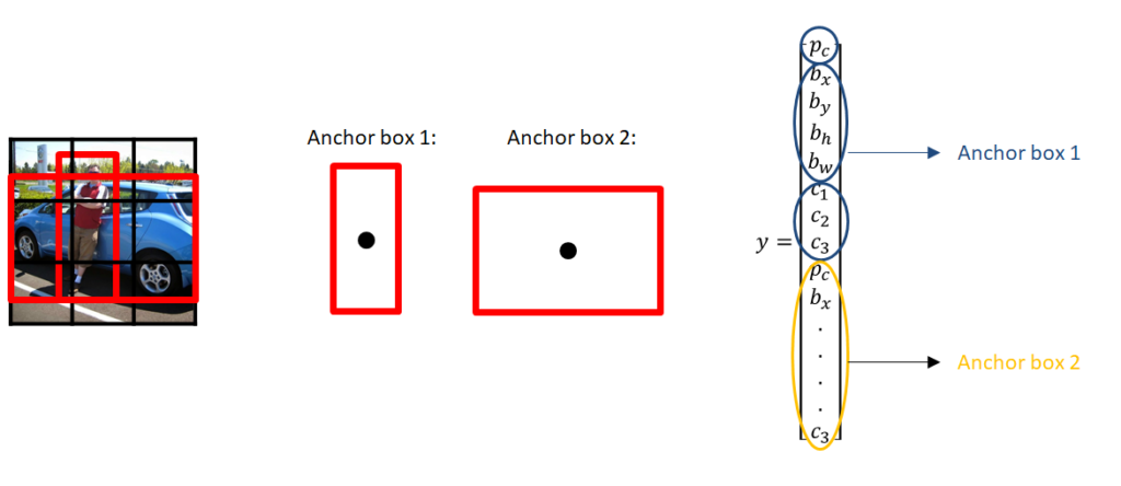
We have a grid and each cell is going to predict:
- For each bounding box:
- \(4\) coordinates (\(t_x, t_ y, t_ w, t_ h\))
- \(1\) objectness error which is confidence score of whether there is an object or not
- Some number of class probabilities
If there is some offset from the top left corner by \(c_x, c_y\), then the predictions correspond to:
$$ b_x = \sigma(t_x) + c_x $$ $$ b_y = \sigma(t_y) + c_y $$ $$ b_w = p_we^{t_w} $$ $$ b_h = p_he^{t_h} $$
Where \(p_w\) and \(p_h\) correspond to bounding box width and height respectively. Instead of predicting offsets like in YOLO V2, the authors predict location coordinates relative to the location of the grid cell.
This output, it is the output of our neural network. In total, there is \(S \times S \times [B * (4 + 1 + C)]\) outputs where \(B\) is the number of bounding boxes predicted by each cell (depends on at how much scales we want our detections to be), \(C\) is the number of classes, \(4\) is for bounding boxes and \(1\) objectness prediction. In one pass we can go from an input image to the output tensor which corresponds to the detections for the image. Also, it is worth mentioning that YOLOv3 predicts boxes at 3 different scales.
Now, if we take the probability and multiply them by the confidence values, we get all of the bounding boxes weighted by their probabilities for containing that object.
Simple thresholding will get us rid of all low confidence value predictions. For the next step, it is important to define what is Intersection Over Union (IoU). The intersection over union computes the size of the intersection and divides it by the size of the union.
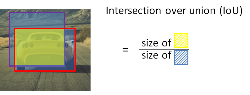
After this, duplicates can still be present and to get rid of them, we apply non-maximum suppression. Non-maximum suppression will take a bounding box with the highest probability and than look at other bounding box that are close to the first one and the ones with the highest overlap with this one (highest IoU) will be suppressed.
Because everything is done in just one pass, it is nearly as fast as classification. Also, all detections are predicted simultaneously, which means that model implicitly incorporates global context. In simpler words, it can learn which objects tend to occur together, relative size and location of objects and so on.

We strongly recommend reading all three Yolo papers:
- You Only Look Once: Unified, Real-Time Object Detection
- YOLO9000: Better, Faster, Stronger
- YOLOv3: An Incremental Improvement
3. Implementation in TensorFlow
The first step in this implementation is to prepare the notebook and import libraries. Here we are using Jupyter Notebooks and all code can be found on Google Colab in the provided link at the end.
In this post we are just going to implement fully convolutional network (FCN) without training. In order to predict something with this network, we need to load weights from a pretrained model. This weights are obtained from training YOLOv3 on Coco (Common Objects in Context) dataset. These weights can be downloaded from the official website.
It is very hard to load weights with pure functional API because the layer ordering is different in tf.keras and darknet. The clean solution here is to create sub-models in keras. TensorFlow Checkpoint is recommended to save nested model as its offically supported by TensorFlow.
Here, we also need to define function for calculating intersection over union. We are using batch normalization to normalize the outputs to speed up learning. tf.keras.layers.BatchNormalization doesn’t work very well for transfer learning, so here is provided another solution to fix this.
At each scale we will define 3 anchor boxes for each grid. In this example the mask is :
- 0,1,2, meaning that we will use the first three anchor boxes
- 3,4,5, meaning that we will use the fourth, fifth and sixth box
- 6,7,8, meaning that we will use the seventh, eighth and ninth box
Now, it is time to implement YOLOv3 network. The main idea here is to use only convolutional layers. There are 53 of them, so the easiest way is to make a function for this, where we will pass important parameters that will change from layer to layer.

Residual Blocks in the YOLOv3 Architecture Diagram is used for feature learning. A Residual Block consists of several convolutional layers and shortcut paths.
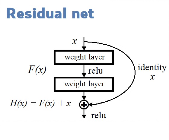
We are building our model using Functional API, which is easy to use. With this, we can easily define branches in our architecture (ResNet block) and easily share layers inside the architecture.
Here, we also define the function for getting rid of duplicates – non maximum suppression.
Function transform targets outputs tuple of shape
(
[N, 13, 13, 3, 6],
[N, 26, 26, 3, 6],
[N, 52, 52, 3, 6]
)
Where \(N\) is the number of labels in batch, and \(6\) represents \([x, y, w, h, obj, class]\) of the bounding boxes.
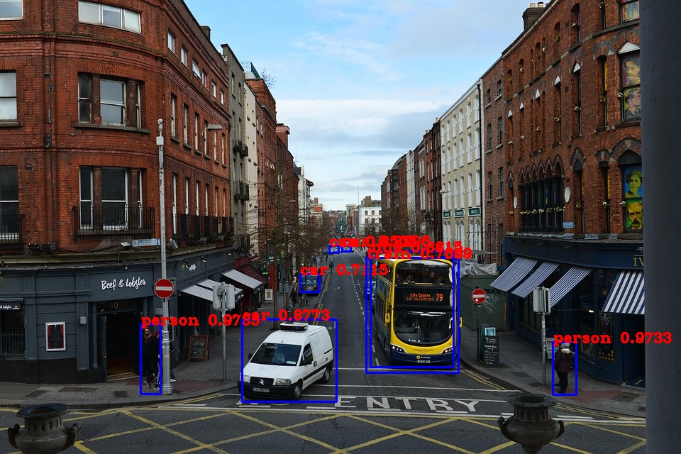
Now, we can create our model, load weights and class names. There is \(80\) of them in Coco dataset. Straight away we can go and test our model with some image.
Let’s see the results.
The interactive Colab notebook with complete code can be found at the following link
Summary
In this post we talked about idea behind YOLOv3 object detection algorithm. We have shown how to implement it using TensorFlow 2.0. In the next post we are going to talk about perspective imaging.