#002 OpenCV projects – How to cartoonize an image with OpenCV in Python?

Highlights: Today you can find countless numbers of photo editing applications on the internet that allows you to transform your images into cartoons on the internet. This pretty cool effect became extremely popular on social media over the past few years. That is why we decided to teach you how to use OpenCV to create your application that can transform an image into a cartoon. To do that we will be working with digital image processing (filters) edges detection algorithms, and color quantization methods. So, let’s begin with our post.

Tutorial overview:

1. Detecting and emphasizing edges
   • Convert the original color image into grayscale
   • Using adaptive thresholding to detect and emphasize the edges in an edge mask. 
   • Apply a median blur to reduce image noise. 
2. Image filtering
   • Apply a bilateral filter to create homogeneous colors on the image. 
3. Creating a cartoon effect
   • Use a bitwise operation to combine the processed color image with the edge mask image
4. Creating a cartoon effect using color quantization

To create a cartoon effect we need to apply the following steps:

1. Detecting and emphasizing edges

To produce accurate carton effects, as the first step, we need to understand the difference between a common digital image and a cartoon image. In the following example, you can see how both images look like.

At the first glance we can clearly see two major differences.

1. The first difference is that the colors in the cartoon image are more homogeneous as compared to the normal image.
2. The second difference is noticeable within the edges that are much sharper and more pronounced in the cartoon.

Now, when we have clarified two main differences it is straightforward what our job is. We need to detect and emphasize the edges and apply a filter to reduce the color palette of the input image. When we achieve that goal, we would obtain a pretty cool result.

Let’s begin by importing the necessary libraries and loading the input image.

# Necessary imports
import cv2
import numpy as np
#  Importing function cv2_imshow necessary for programming in Google Colab
from google.colab.patches import cv2_imshowCode language: PHP (php)

Now, we are going to load the image.

img = cv2.imread("Superman.jpeg")
cv2_imshow(img)Code language: JavaScript (javascript)

The next step is to detect the edges. For that task, we need to choose the most suitable method. Remember, our goal is to detect clear edges. There are several edge detectors that we can pick. Our first choice will be one of the most common detectors, and that is the Canny edge detector. But unfortunately, if we apply this detector we will not be able to achieve desirable results. We can proceed with Canny, and yet you can see that there are too many details captured. This can be changed if we play around with Canny’s input parameters (numbers 100 and 200).

edges = cv2.Canny(img, 100, 200)
cv2_imshow(edges)

Although Canny is an excellent edge detector that we can use in many cases in our code we will use a threshold method that gives us more satisfying results. It uses a threshold pixel value to convert a grayscale image into a binary image. For instance, if a pixel value in the original image is above the threshold, it will be assigned to 255. Otherwise, it will be assigned to 0 as we can see in the following image.

However, a simple threshold may not be good if the image has different lighting conditions in different areas. In this case, we opt to use cv2.adaptiveThreshold() function which calculates the threshold for smaller regions of the image. In this way, we get different thresholds for different regions of the same image. That is the reason why this function is very suitable for our goal. It will emphasize black edges around objects in the image.

So, the first thing that we need to do is to convert the original color image into a grayscale image. Also, before the threshold, we want to suppress the noise from the image to reduce the number of detected edges that are undesired. To accomplish this, we will apply the median filter which replaces each pixel value with the median value of all the pixels in a small pixel neighborhood. The function cv2.medianBlur()requires only two arguments: the image on which we will apply the filter and the size of a filter. A more detailed explanation about filters you can find in the book “The hundred-page Computer Vision OpenCV book in Python”.

The next step is to apply cv2.adaptiveThreshold()function. As the parameters for this function we need to define:

• max value which will be set to 255
• cv2.ADAPTIVE_THRESH_MEAN_C : a threshold value is the mean of the neighbourhood area.
• cv2.ADAPTIVE_THRESH_GAUSSIAN_C : a threshold value is the weighted sum of neighbourhood values where weights are a gaussian window.
• Block Size – It determents the size of the neighbourhood area.
• C – It is just a constant which is subtracted from the calculated mean (or the weighted mean).

For better illustration, let’s compare the differences when we use a median filter, and when we do not apply one.

gray = cv2.cvtColor(img, cv2.COLOR_BGR2GRAY)
edges = cv2.adaptiveThreshold(gray, 255, cv2.ADAPTIVE_THRESH_MEAN_C, cv2.THRESH_BINARY, 9, 5)

gray = cv2.cvtColor(img, cv2.COLOR_BGR2GRAY)
gray_1 = cv2.medianBlur(gray, 5)
edges = cv2.adaptiveThreshold(gray_1, 255, cv2.ADAPTIVE_THRESH_MEAN_C, cv2.THRESH_BINARY, 9, 5)

As you can see we will obtain much better results when we apply a median filter. Naturally, edge detection obviously is not perfect. One idea that we will not explore here and that you can try on your own is to apply morphological operations on these images. For instance, erosion can assist us here to eliminate small tiny lines that are not a part of a large edge.

2. Image filtering

Now we need to choose a filter that is suitable for converting an RGB image into a color painting or a cartoon. There are several filters that we can use. For example, if we choose to use cv2.medianBlur() filter we will obtain a solid result. We will manage to blur the colors of the image so that they appear more homogeneous. On the other hand, this filter will also blur the edges and this is something that we want to avoid.

The most suitable filter for our goal is a bilateral filter because it smooths flat regions of the image while keeping the edges sharp.

Bilateral filter

Bilateral filter is one of the most commonly used edge-preserving and noise-reducing filters. In the following image you can see an example of a bilateral filter in 3D when it is processing an edge area in the image.

Similarly to the Gaussian, bilateral filter replaces each pixel value with a weighted average of nearby pixel values. However, the difference between these two filters is that a bilateral filter takes into account the variation of pixel intensities in order to preserve edges. The idea is that two nearby pixels that occupy nearby spatial locations also must have some similarity in the intensity levels. To better understand this let’s have a look in the following equation:

$$ BF[I]_{\mathbf{p}}=\frac{1}{W_{\mathbf{p}}}\sum_{\mathbf{q}\in\mathcal{S}}G_{\sigma_{s}}(\|\mathbf{p}-\mathbf{q}\|)G_{\sigma_{r}}\left(I_{\mathbf{p}}-I_{\mathbf{q}}\right) I_{\mathbf{q}} $$

Were:

$$ W_{\mathbf{p}}=\sum_{\mathbf{q}\in\mathcal{S}}G_{\sigma_{s}}(\|\mathbf{p}-\mathbf{q}\|)G_{\sigma_{r}}\left(I_{\mathbf{p}}-I_{\mathbf{q}}\right) $$

Here, the term \(\frac{1}{W_{p}} \) is a normalized weighted average of nearby pixels \(p \) and \(q \). Parameters \(\sigma_{s} \) and \(\sigma_{r} \) control the amount of filtering. \(G_{\sigma_{s}} \) is a spatial Gaussian function that controls the influence of distant pixels, and \(G_{\sigma_{r}} \) is a range Gaussian function that controls the influence of pixels with an intensity value different from the central pixel intensity \(I_{p} \). So, this function makes sure that only those pixels with similar intensities to the central pixel are considered for smoothing. Therefore, it will preserve the edges since pixels at edges will have large intensity variation. 

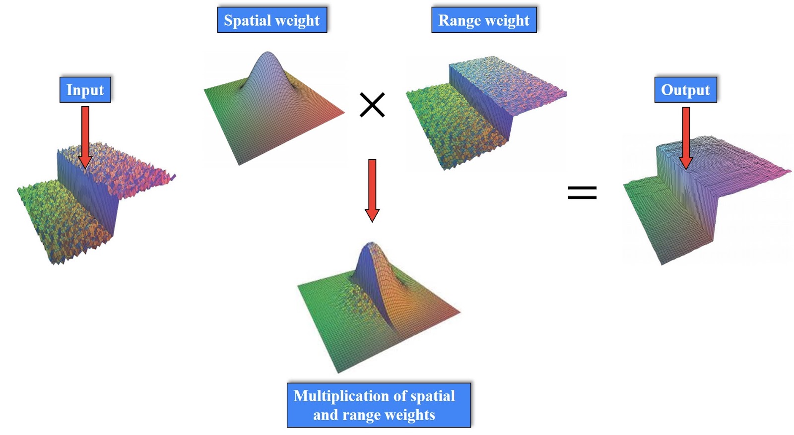
Now, to visualize this equation let’s have a look at the following image. On the left we have an input image represented in 3D. We can see that it has one sharp edge. Then, we have a spatial weight and a range weight function based on pixel intensity. Now, when we multiply range and spatial weights we will get a combination of these weights. In that way the output image will still preserve the sharp edges while flat areas will be smoothed.

There are three arguments in cv2.bilateralFilter() function:

• d – Diameter of each pixel neighborhood that is used during filtering.
• sigmaColor – the standard deviation of the filter in the color space. A larger value of the parameter means that farther colors within the pixel neighborhood will be mixed together, resulting in larger areas of semi-equal color.
• sigmaSpace –the standard deviation of the filter in the coordinate space. A larger value of the parameter means that farther pixels will influence each other as long as their colors are close enough.

color = cv2.bilateralFilter(img, d=9, sigmaColor=200,sigmaSpace=200)
cv2_imshow(color)

3. Creating a cartoon effect

Our final step is to combine the previous two: We will use cv2.bitwise_and() the function to mix edges and the color image into a single one. If you need a more detailed explanation about bitwise operations click on this link.

cartoon = cv2.bitwise_and(color, color, mask=edges)
cv2_imshow(cartoon)

This is our final result, and you can see that indeed we do get something similar to a cartoon or a comic book image. Would you agree that this looks like Superman from colored comic books?

4. Creating a cartoon effect using color quantization

Another interesting way to create a cartoon effect is by using the color quantization method. This method will reduce the number of colors in the image and that will create a cartoon-like effect. We will perform color quantization by using the K-means clustering algorithm for displaying output with a limited number of colors.

First, we need to define color_quantization() function.

def color_quantization(img, k):
# Defining input data for clustering
  data = np.float32(img).reshape((-1, 3))
# Defining criteria
  criteria = (cv2.TERM_CRITERIA_EPS + cv2.TERM_CRITERIA_MAX_ITER, 20, 1.0)
# Applying cv2.kmeans function
  ret, label, center = cv2.kmeans(data, k, None, criteria, 10, cv2.KMEANS_RANDOM_CENTERS)
  center = np.uint8(center)
  result = center[label.flatten()]
  result = result.reshape(img.shape)
  return resultCode language: PHP (php)

Different values for \(K \) will determine the number of colors in the output picture. So, for our goal, we will reduce the number of colors to 7. Let’s look at our results.

img_1 = color_quantization(img, 7)
cv2_imshow(img_1)

Not bad at all! Now, let’s see what we will get if we apply the median filter on this image. It will create more homogeneous pastel-like coloring.

blurred = cv2.medianBlur(img_1, 3)
cv2_imshow(blurred)

And finally, let’s combine the image with detected edges and this blurred quantized image.

cartoon_1 = cv2.bitwise_and(blurred, blurred, mask=edges)
cv2_imshow(cartoon_1)

For better comparison let’s take a look at all our outputs.

So, there you go. You can see that our Superman looks pretty much like a cartoon superhero.

Before you go: You can treat this post as a learning playground. On many occasions, there is no magic wand that will work the best for all images and superheros. It is you who will determine, what combination of filtering, edges, blurring, color quantization will produce the best results for your project. That’s why CV can be so creative!

Summary

In this post, we learned how to apply edge detection and image filtering to achieve a cool cartoon effect. Moreover, we also showed how the color quantization method can also be used for this purpose. The next post will also be a funny one. We will teach you to detect different parts of the face, and overlay them with a funny objects like masks, mustashes and glasses.

References:

[1] OpenCV – Python tutorials

[2] OpenCV: Computer Vision Projects with Python by Joseph Howse, Prateek Joshi, Michael Beyeler

[3] How to create a cartoon effect – Opencv with Python by Sergio Canu