#015 TF Implementing AlexNet in TensorFlow 2.0
Highlights: In this post we will show how to implement a fundamental Convolutional Neural Network \(AlexNet\) in TensorFlow 2.0. The AlexNet architecture is designed by Alex Krizhevsky and published with Ilya Sutskever and Geoffrey Hinton. It competed in the ImageNet Large Scale Visual Recognition Challenge in 2012.
Tutorial Overview:
1. Review of the Theory
Real life Computer Vision problems requires big amount of quality data to be trained on. In the past, people were using CIFAR and NORB dataset as a benchmark datasets for Computer Vision problems. However, the ImageNet competition changed that. This dataset required a more complex network than before in order to achieve good results.
One network architecture which achieved the best result back in 2012 was AlexNet. It achieved a Top-5 error rate of 15.3%. The next best result was far behind (26.2%).
This architecture has around 60 million parameters and consists of the following layers.
| Layer Type | Feature Map | Size | Kernel Size | Stride | Activation |
|---|---|---|---|---|---|
| Image | 1 | 227×227 | – | – | – |
| Convolution | 96 | 55×55 | 11×11 | 4 | ReLU |
| Max Pooling | 96 | 27×27 | 3×3 | 2 | – |
| Convolution | 256 | 27×27 | 5×5 | 1 | ReLU |
| Max Pooling | 256 | 13×13 | 3×3 | 2 | – |
| Convolution | 384 | 13×13 | 3×3 | 1 | ReLU |
| Convulution | 384 | 13×13 | 3×3 | 1 | ReLU |
| Convulution | 256 | 13×13 | 3×3 | 1 | ReLU |
| Max Pooling | 256 | 6×6 | 3×3 | 2 | – |
| Fully Connected | – | 4096 | – | – | ReLU |
| Fully Connected | – | 4096 | – | – | ReLU |
| Fully Connected | – | 1000 | – | – | Softmax |
In our case, we will train a model on only two classes from ImageNet dataset, so our last Fully Connected layer will have only two neurons with Softmax activation function.
There are a few changes which made AlexNet differ from other networks back in the time. Let’s see what changed the history!
Overlapping pooling layers
Standard pooling layers are summarizing the outputs of neighboring groups of neurons in the same kernel map. Traditionally, the neighborhoods summarized by adjacent pooling units do not overlap. Overlapping pooling layers are similar to the standard pooling layers, except the adjacent windows over which the Max is computed overlap each other.

ReLU nonlinearity
Traditional way to evaluate a neuron output is using \(sigmoid\) or \(tanh\) activation function. These two functions are fixed between min and max value, so they are saturating nonlinear. However, in AlexNet, Rectified linear unit function, or shortly \(ReLU\) is used. This function has a threshold at \(0\). This is a nonsaturating activation function.
\(ReLU\) function requires less computation and allows faster learning, which has a great influence on the performance of large models trained on large datasets.
Local Response Normalization
Local Response Normalization (LRN) was first introduced in AlexNet architecture where the activation function of choice was \(ReLU\). The reason for using LRN was to encourage lateral inhibition. This refers to the capacity of a neuron to reduce the activity of its neighbors. This is useful when we are dealing with neurons with \(ReLU\) activation function. Neurons with \(ReLU\) activation function have unbounded activations and we need LRN to normalize that.
2. Implementation in TensorFlow 2.0
The interactive Colab notebook can be found at the following link
Let’s start with importing all necessary libraries.
After imports, we need to prepare our data. Here, we will use only a small part of the ImageNet dataset. With the following code you can download all images and store them in folders.
Now we can create a network. Last layer in the original \(AlexNet\) has 1000 neurons, but here we will use only one. That is because we will use images for only two classes. In order to build our convolutional neural network we will use the Sequential API.

After creating a model, let’s define some important parameters for later use. In addition, let’s create Image Data Generators. \(AlexNet\) has a lot of parameters, 60 million, which is a huge number. This will make overfitting highly possible if there are not sufficient data. So here, we will make use of a data augmentation technique, about which you can find more here.
For the same reason, dropout layers are used in \(AlexNet\). This technique consists of “turning off” neurons with a predetermined probability. This forces each neuron to have more robust features that can be used with other neurons. We won’t use a dropout layers here because we won’t use the whole dataset.
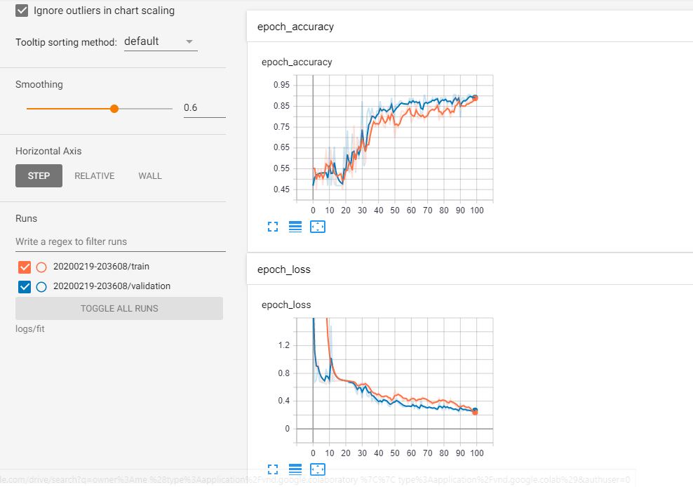
Now we can set up the TensorBoard and start training our model. This way we can track the model performance in real-time.
Let’s use our model to make some predictions and visualize them.

Summary
In this post we showed how to implement \(AlexNet\) in TensorFlow 2.0. We were using just a part of the ImageNet dataset, and that is why we did not get the best results. For better accuracy, more data and longer training time is required.