LLM_log #038: Policy Gradients — From Imitation to REINFORCE

Policy Gradients — From Imitation to REINFORCE
Highlights: SFT can only copy demonstrations and never learns from failure; REINFORCE instead weights every sampled run by its reward, and with 0/1 rewards it becomes SFT on the successes. Daniel Fried’s lecture in CMU 11-768 AI Agents (Fall 2026) analyzes the limitations of supervised fine-tuning and establishes interactive reinforcement learning formulations for language agents. Using a pedagogical Number Search environment, we walk through POMDP trajectories, exposure bias, and the expert-iteration loop of Reinforced Self-Training (ReST). We then cover the five-step derivation of REINFORCE and show how token masking and binary reward scaling connect policy gradients directly to standard cross-entropy loss.
- Supervised training limits: Next-token imitation suffers from task mismatch by penalizing valid alternative paths identically to disastrous errors, while discarding failed trajectories that contain critical boundary feedback.
- Exposure bias: Agents trained solely on pristine expert demonstrations fail to recover when autoregressive errors produce unfamiliar, out-of-distribution conditioning states.
- Reinforced self-training: ReST alternates between sampling rollouts from current policy weights, filtering traces via verified rewards, and running supervised updates strictly on passing executions.
- Dynamics cancellation: Applying the log-derivative trick within REINFORCE cancels non-differentiable external environment transition dynamics, isolating policy action parameters for optimization.
- Loss equivalence: Weighting token-masked cross-entropy loss by binary scalar rewards renders online policy gradients algebraically identical to offline filtered self-training.
Tutorial Overview:
- The Number Search Environment
- Limits of Supervised Fine-Tuning
- Formulating the Agent-Environment Loop and Trajectories
- Reinforced Self-Training (ReST)
- Deriving the Policy Gradient: REINFORCE
- Scaling and Masking SFT Loss
- Summary
1. The Number Search Environment
In short
– Number Search tests an agent’s ability to guess hidden integers within four attempts.
– Different search trajectories can achieve identical target numbers and earn full binary rewards.
– Verified rewards evaluate trajectories using binary or continuous success metrics like unit tests.
1.1 Task Mechanics and Feedback Loops
Daniel Fried introduces Number Search as a toy problem illustrating fundamental reinforcement learning mechanics.
- 1 to 16: hidden secret integer range unknown to the searching agent.
- 4 guesses: maximum guess budget allowed before the environment forces episode termination.
- Directional feedback: sequential environment clues of higher, lower, or correct returned after each guess.
- Interactive cycle: four-step interaction loop continuing until target discovery or guess budget exhaustion.
- The agent submits a numerical guess between 1 and 16.
- The environment compares the guess to the hidden target.
- The agent receives directional feedback of higher, lower, or correct.
- The cycle repeats until the agent discovers 11 or times out.
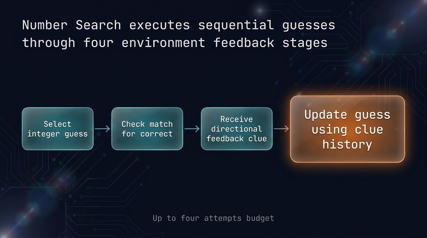
Fig 1. A four-step interaction cycle gives directional feedback until the agent discovers the target.
Finite guess limits force agents to search efficiently under tight budgets. Directional clues reward targeted narrowing over random guessing.
1.2 Candidate Trajectories and Search Strategies
Agents generate a trajectory (a complete sequential rollout recording all observations, agent actions, and intermediate rewards across an episode).
- 11 target: specific hidden number used to evaluate diverse candidate agent policies.
- Trajectory 1: 8, 12, 10, and 11 execute optimal binary search to reach success.
- Trajectory 2: 4, 8, 12, and 11 adapt from a suboptimal guess to succeed.
- Trajectory 3: 16, 8, 9, and 10 end in timeout after an extreme start.
- Trajectory 4: 1, 2, 3, and 4 fail by executing an ineffective linear search.
- Positive task rewards: identical maximum returns earned by trajectories 1 and 2 despite divergent paths.
| Trajectory | Search Strategy | Guesses and Feedback | Outcome |
|---|---|---|---|
| $\tau_1$ | Binary search | 8 (higher), 12 (lower), 10 (higher), 11 (correct) | Discovered ($R=1$) |
| $\tau_2$ | Adaptive recovery | 4 (higher), 8 (higher), 12 (lower), 11 (correct) | Discovered ($R=1$) |
| $\tau_3$ | Extreme bound | 16 (lower), 8 (higher), 9 (higher), 10 (timeout) | Timeout ($R=0$) |
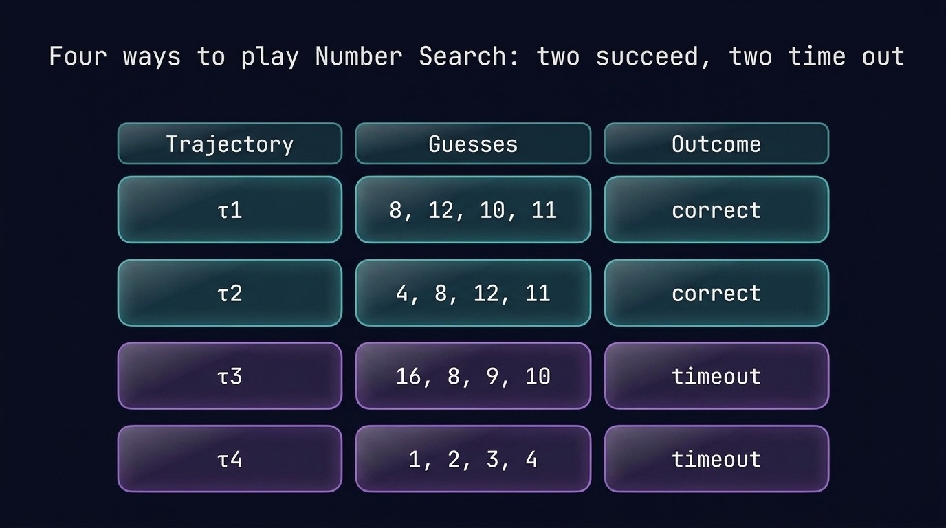
Fig 2. Different action sequences discover the secret target and achieve identical positive task rewards.
Different policies explore distinct paths because agents balance exploration and recovery. Reinforcement learning credits overall task success rather than specific paths taken.
1.3 Reward Structure and Benchmark Verification
Tasks use RLVR (a reinforcement learning setting where rewards are evaluated through verifiable outcomes, such as passing unit tests).
- Scalar rewards: single numerical values measuring how good or bad a completed trajectory was.
- R = 1: binary reward granted for identifying the number within four guesses.
- R = 0: zero reward assigned when an agent exhausts guesses and times out.
- SWE-bench: real-world benchmark rewarding 1 if an agent patch passes all unit tests.
- Continuous rewards: fractional percentages of passed unit tests extending beyond simple binary rewards.
- Direct RL applicability: core reinforcement learning algorithms handle binary and arbitrary scalar rewards identically.
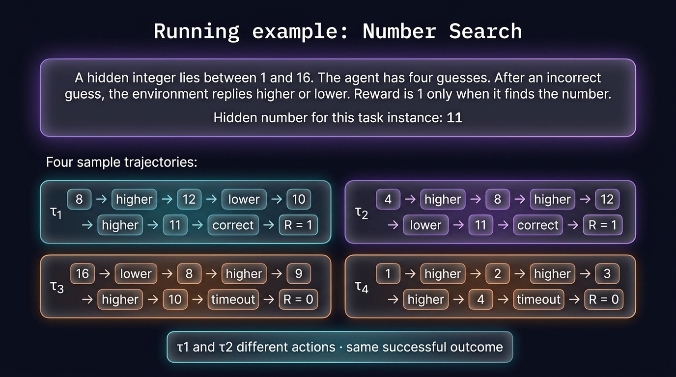
Fig 3. Daniel Fried’s Number Search lecture slide illustrates search bounds, guess counts, and feedback.
Verified unit tests prevent reward gaming by providing objective ground truth. Scalar feedback algorithms generalize cleanly across discrete and continuous metrics.
2. Limits of Supervised Fine-Tuning
In short
– Supervised fine-tuning copies target tokens rather than optimizing end-to-end task completion.
– Pristine demonstration data leaves agents incapable of recovering from generation mistakes.
– Discarding failed interaction rollouts wastes critical feedback about catastrophic actions.
2.1 Supervised Fine-Tuning on Demonstration Histories
Supervised fine-tuning (SFT) [Training an agent to imitate a given task demonstration by copying demonstrated actions and maximizing their sequence probability.] trains an agent to reproduce target demonstration actions.
- Human demonstrations: experts manually write or execute step-by-step target trajectories.
- Model distillation: a larger, more capable teacher model generates the reference traces.
- Self-generated traces: the agent executes runs and filters out successful interaction histories.
- 1 to 16 search space: the environment hides a secret integer between 1 and 16, which is unknown to the agent.
- Alternating tokens: interaction histories interleave prompt tokens, agent guesses, and environmental feedback messages.
- Secret target 11: target demonstration (\tau_1) executes guesses 8, 12, 10, and terminates on 11.
Agents train strictly on recorded observations without discovering whether alternative guesses also succeed. Imitating specific sequences prevents policy exploration.
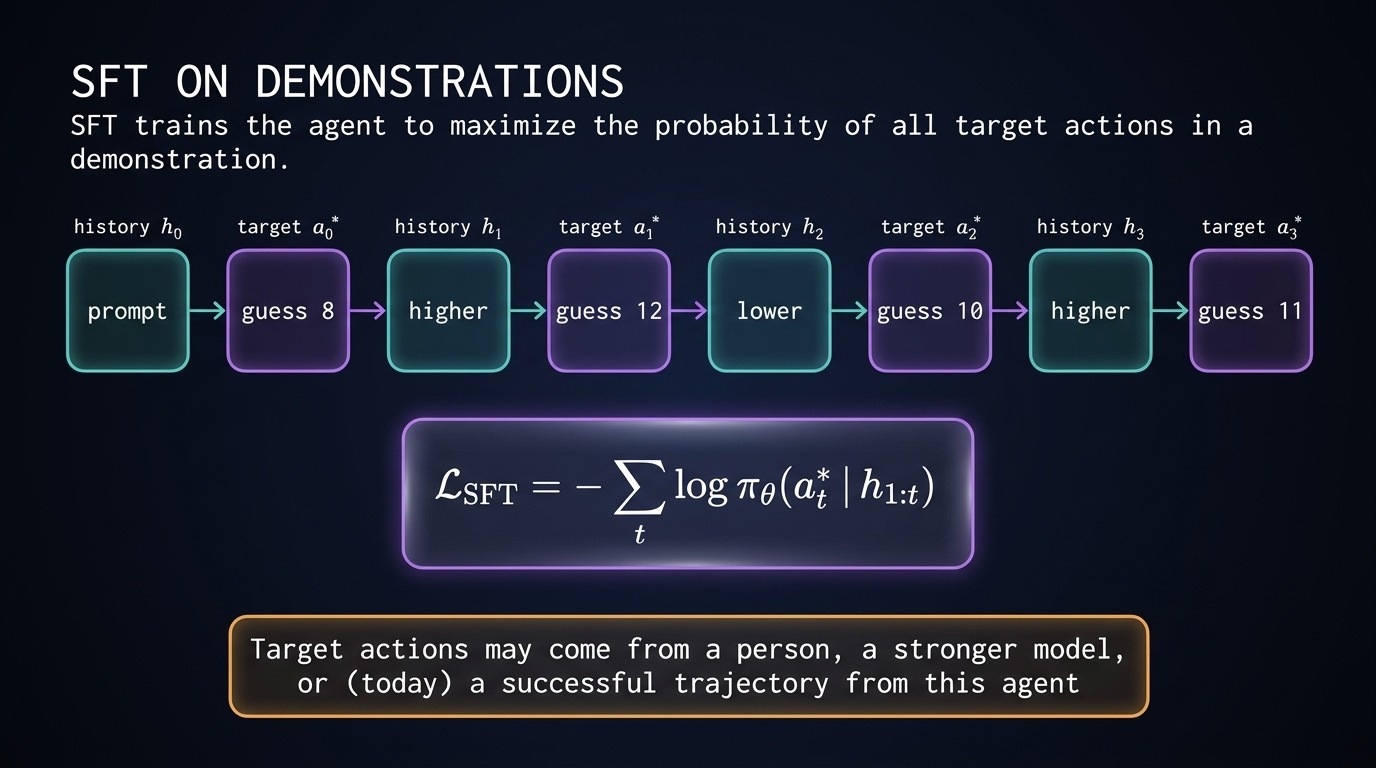
Fig 4. Supervised training optimizes next-token prediction over pre-recorded expert demonstration histories.
2.2 Mathematical Objective of Demonstration Training
Supervised objectives minimize standard sequence cross-entropy loss over target tokens conditioned on preceding history tokens.
- History context (h_{1:t}): the complete sequence of environment feedback and past actions up to step (t).
- Target action (a_t^*): the exact ground-truth demonstration token selected for execution at step (t).
- Parameterized policy (\pi_\theta): the neural network predicting the probability distribution over candidate next tokens.
- Loss formulation: the objective minimizes negative log-likelihood across all sequential target demonstration steps.
[\mathcal{L}{\text{SFT}} = – \sum_t \log \pi\theta(a_t^* \mid h_{1:t})]
- Token-level penalty: the loss penalizes any deviation from demonstrated tokens regardless of outcome quality.
Supervised loss operates purely at the token level. It cannot measure whether alternative token choices achieve the same goal.
2.3 Task Mismatch in Policy Optimization
Task mismatch [A disconnect where an algorithm optimizes matching specific demonstrated tokens rather than achieving overall successful task completion.] creates a divergence between token imitation and task success.
- Goal divergence: maximizing token probability does not equal maximizing task completion probability.
- Multiple paths: the secret number 11 can be found via alternative valid guess sequences.
- Path (\tau_2): guessing 4, then 8, 12, and 11 reaches the correct secret integer successfully.
- Equal penalty: guessing reasonable 4 receives the same cross-entropy loss penalty as guessing disastrous 13.
- Asymmetric errors: guessing lower than 8 after receiving “higher” constitutes a fatal reasoning error.
Supervised losses assign zero credit to valid alternate solutions. They blindly penalize any deviation from the single recorded demonstration.
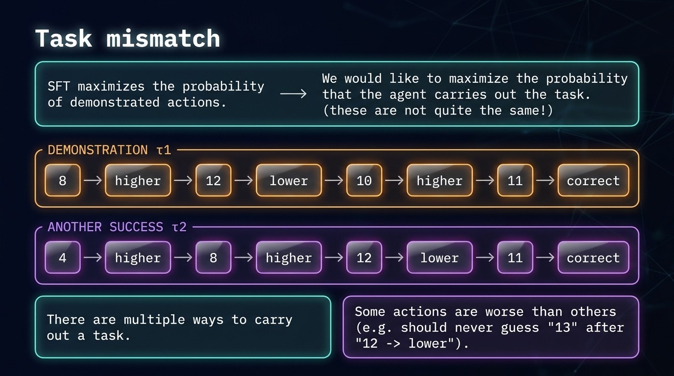
Fig 5. Task mismatch penalizes valid alternative successful solutions identical to fatal mistakes.
2.4 Evaluating Valid Actions Against Targets
Demonstrations represent only one path through the state space, ignoring decision quality differences across choices.
| Candidate Action | Environment State | Action Quality | Training Loss |
|---|---|---|---|
| Guess 8 | Start of episode | Demonstrated target | Zero penalty |
| Guess 4 | Start of episode | Valid alternative | Maximum penalty |
| Guess 13 | Feedback was “lower than 12” | Disastrous mistake | Maximum penalty |
- Identical loss values: cross-entropy treats sensible alternative guess 4 exactly like catastrophic guess 13.
- Zero search awareness: the model never learns that multiple numbers narrow down the interval.
- Target rigidity: the policy overfits to specific sequences observed during training runs.
Models must distinguish catastrophic actions from sensible alternatives. Token cross-entropy cannot differentiate these outcome qualities.
2.5 Data Mismatch from Suboptimal Trajectories
Data mismatch prevents standard supervised fine-tuning from learning valuable negative lessons from failed environment trajectories [A complete sequential rollout recording all observations, agent actions, and intermediate rewards across an episode.].
- Trajectory (\tau_1): guesses 8, 12, 10, and 11 to achieve a successful task outcome.
- Trajectory (\tau_2): guesses 4, 8, 12, and 11 to achieve a successful task outcome.
- Trajectory (\tau_3): guesses 16, 8, 9, and 10, terminating in a timeout failure.
- Trajectory (\tau_4): increments guesses 1, 2, 3, and 4, also hitting an episode timeout.
- Discarded data: standard SFT drops (\tau_3) and (\tau_4) entirely to avoid imitating bad guesses.
- Lost information: failed rollouts contain critical negative signals showing which search actions cause timeouts.
Directly imitating failed runs teaches agents poor reasoning habits. Discarding suboptimal runs wastes valuable information about fatal boundaries.
2.6 Autoregressive Rollouts and Exposure Bias
Exposure bias [A training flaw where an agent exposed only to pristine demonstrations cannot recover when it makes an error during autoregressive generation.] leaves agents unprepared for errors during inference rollouts.
- The agent samples initial action (a_0) using prompt history (h_0).
- The environment evaluates the action and returns intermediate observation (h_1).
- The model appends action (a_0) and feedback (h_1) to create conditioning history (h_{1:2}).
- The agent samples next action (a_1) autoregressively from its current output distribution.
- The loop repeats until the agent outputs a terminal guess or times out.
- Pristine histories: training feeds strictly ground-truth demonstrations into model context windows.
- Compounding drift: one uncalibrated guess produces an unseen history context during test-time rollouts.
- Disorientation: an agent guessing 2 after “higher than 8” enters unfamiliar, out-of-distribution states.
- Cascading failures: the policy cannot recover from self-generated errors and outputs repetitive mistakes.
Training exclusively on perfect demonstrations guarantees brittleness. The agent never encounters corrupted states during training.
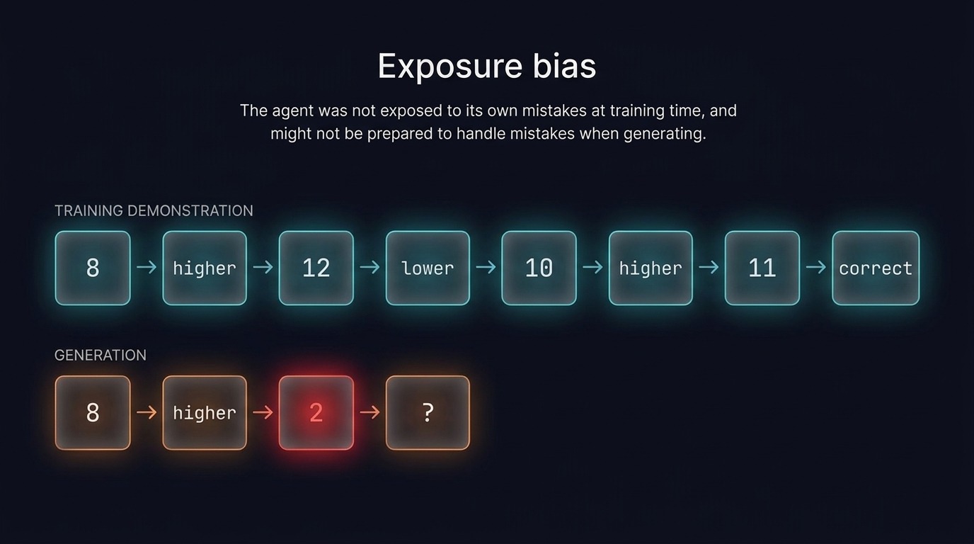
Fig 6. Autoregressive rollouts drift into unfamiliar distribution states when agents make unrecoverable errors.
2.7 Remediating Exposure Bias Through Reinforcement
Interactive reinforcement learning exposes agents to self-generated states, teaching active recovery from suboptimal execution steps.
- On-policy generation: interaction rollouts sample actions directly from the agent’s current active policy during training [On-policy].
- Error exploration: agents encounter mistakes during training rollouts and observe resulting environment feedback.
- Recovery learning: the policy discovers actions that steer corrupted interaction states back toward success.
- Outcome rewards: feedback scores complete trajectories rather than forcing adherence to demonstrated token sequences.
On-policy sampling forces agents to navigate the consequences of their mistakes. Policies learn robust recovery strategies.
3. Formulating the Agent-Environment Loop and Trajectories
In short
– Reinforcement learning replaces fixed demonstrations with interactive trial-and-error policy optimization.
– Agents act under partial observability, conditioning solely on visible interaction history.
– Optimization maximizes expected return by shifting probability mass to winning trajectories.
3.1 Overcoming Supervised Learning Pitfalls
Reinforcement learning lets models generate their own actions and collect environmental rewards rather than copying static demonstration datasets.
- Direct reward optimization: targets task completion directly instead of maximizing surrogate token probabilities.
- Task mismatch [A disconnect where an algorithm optimizes matching specific demonstrated tokens rather than achieving overall successful task completion]: fixes token-level imitation gaps by rewarding overall successful episode outcomes.
- Active error correction: collects positive feedback from successes and negative feedback from failures.
- Exposure bias [A training flaw where an agent exposed only to pristine demonstrations cannot recover when it makes an error during autoregressive generation]: trains policies on-policy [Sampling interaction rollouts directly from the agent’s current active policy during training rather than from pre-recorded datasets] to learn recovery behavior from self-generated mistakes.
- Loop elimination: resolves degenerative repetition patterns common in supervised fine-tuning (SFT) [Training an agent to imitate a given task demonstration by copying demonstrated actions and maximizing their sequence probability].
| Problem Mode | Supervised Fine-Tuning | Reinforcement Learning |
|---|---|---|
| Optimization Target | Demonstration token likelihood | Expected trajectory return |
| Data Generation | Fixed offline traces | Dynamic on-policy rollouts |
| Error Handling | Compounding off-distribution drift | Real-time state recovery |
Supervised imitation suffers when test distributions drift away from expert demonstrations. Direct interaction forces models to discover stabilizing paths when unexpected errors occur.
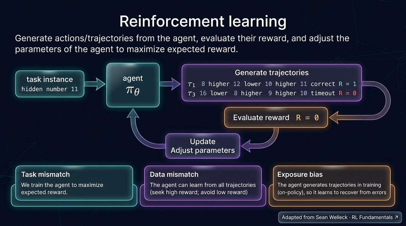
Fig 7. Reinforcement learning guides parameter updates by scoring model-generated actions through environment interactions.
3.2 POMDP Formulation and History Conditioning
Because the environment hides a secret integer between 1 and 16, which is unknown to the agent, the task forms a partially observable Markov decision process (POMDP) [A decision environment where true underlying states are hidden, requiring the agent to act purely based on visible interaction history].
- Invisible underlying states: conceals true world configurations, such as hidden server databases or target numbers.
- Conditioned history sequence: builds visible step records $h_t = (o_0, a_0, o_1, \dots, o_t)$ across time.
- Action distribution: samples discrete outputs directly from language model parameters via $\pi_\theta(a_t \mid h_t)$.
- Full rollout trajectory [A complete sequential rollout recording all observations, agent actions, and intermediate rewards across an episode]: stores complete interaction episodes $\tau = (o_0, a_0, r_1, o_1, \dots, a_{T-1}, r_T, o_T)$.
- Cumulative return formula: sums intermediate episode scalar feedback through $R(\tau) = \sum_{t=1}^T r_t$.
- 0 or 1 terminal return: awards 1 for guessing the secret integer and 0 for timeouts.
Under partial observability, policies cannot condition on hidden world states. Agents must decide their next action based strictly on visible dialogue histories.
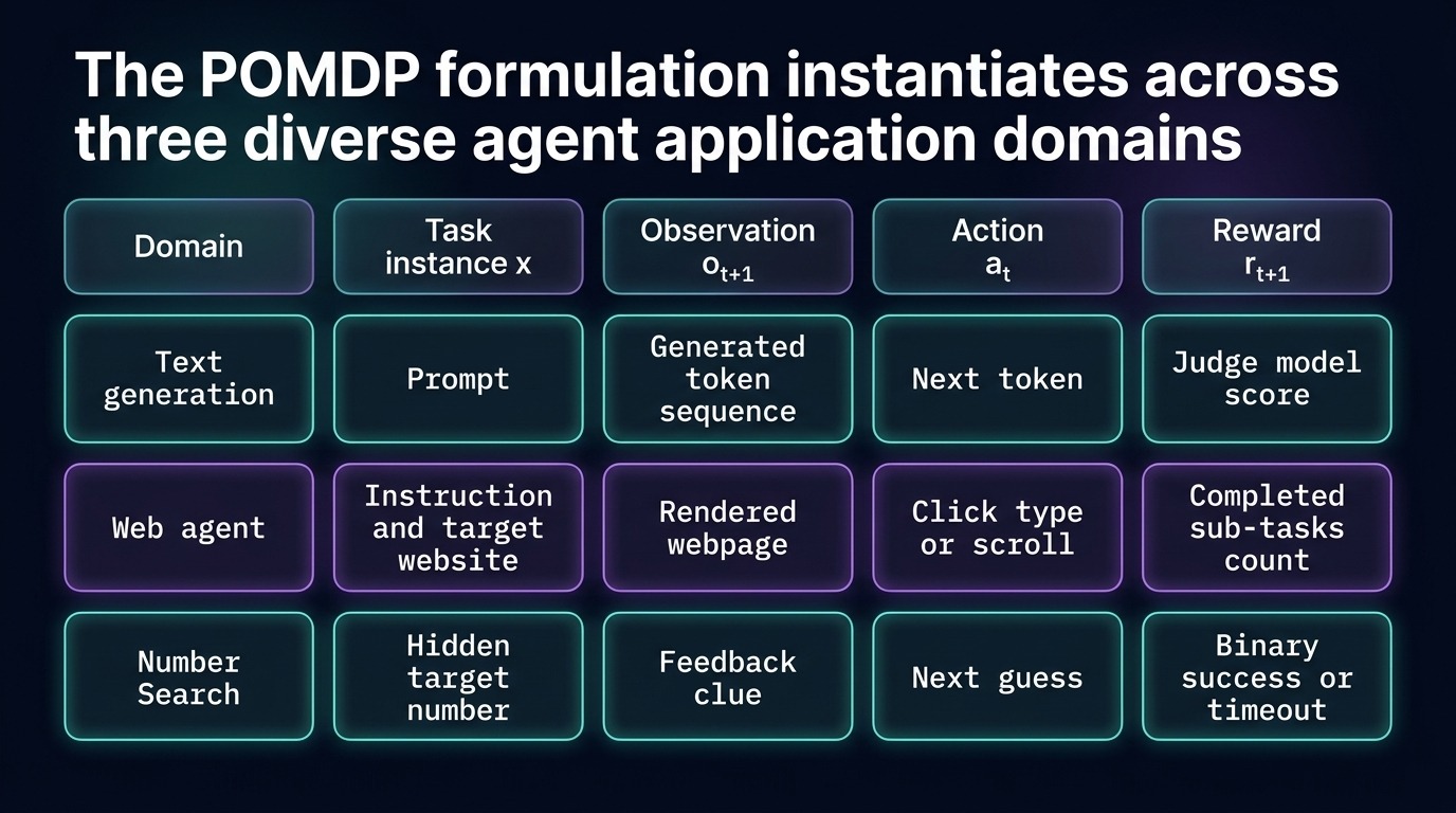
Fig 8. POMDP agents condition their next actions on visible interaction histories rather than hidden states.
3.3 Factoring Trajectories with Unknown Dynamics
The joint probability of a trajectory combines model policy decisions with stochastic transition dynamics from the external environment.
- Trajectory probability decomposition: factors distributions into $p_\theta(\tau \mid x) = \prod_t \pi_\theta(a_t \mid h_t) P(o_{t+1}, r_{t+1} \mid h_t, a_t, x)$.
- Policy action factor: evaluates token probabilities $\pi_\theta(a_t \mid h_t)$ parameterized by network weights $\theta$.
- Environment transition distribution: governs next observations and scalar rewards through unknown world dynamics $P$.
- Model-free sampling: interacts directly with environments to collect empirical rollouts without knowing closed-form dynamics.
- Parameter gradient updates: leverages empirical trajectory samples to compute policy updates despite unknown transition functions.
Complex external environments lack closed-form equations for page layouts or code execution engines. Empirical rollouts circumvent unknown dynamics through active environmental sampling.
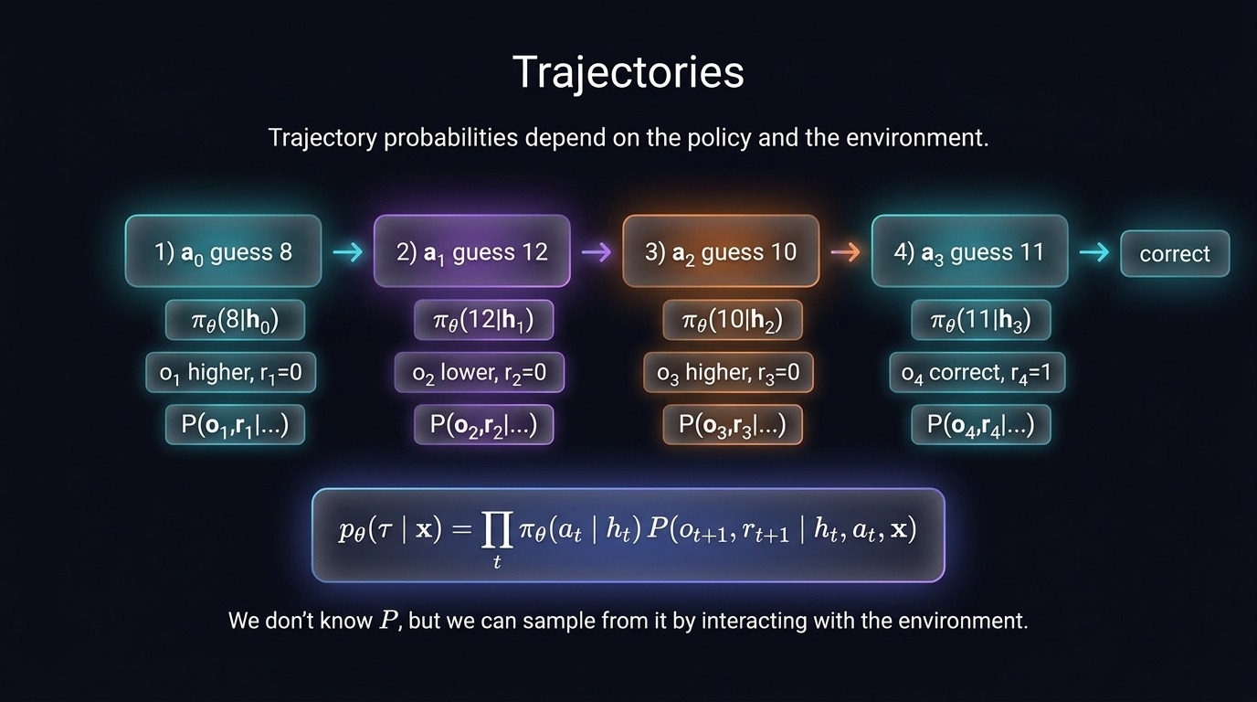
Fig 9. Trajectory probabilities factor into an alternating product of policy decisions and environment transitions.
3.4 Maximizing the Expected Reward Objective
Policy training formalizes learning as an optimization problem that maximizes expected return across all sampled rollouts.
- Sample interaction trajectory $\tau$ from the current policy distribution $p_\theta(\cdot \mid x)$.
- Calculate total episode return $R(\tau)$ using verifiable reward functions.
- Compute expected reward objective $J(\theta) = \mathbb{E}{\tau \sim p\theta(\cdot \mid x)} [R(\tau)]$.
- Shift policy probability mass away from zero-reward traces toward successful trajectories.
- 0.50 expected baseline return: averages discrete trajectory outcomes over four candidate paths.
- 0.30 probability for $\tau_1$: yields success with reward $R(\tau_1) = 1$.
- 0.20 probability for $\tau_2$: yields success with reward $R(\tau_2) = 1$.
- 0.25 probability for $\tau_3$: yields failure with reward $R(\tau_3) = 0$.
- 0.25 probability for $\tau_4$: yields failure with reward $R(\tau_4) = 0$.
Gradient updates increase the likelihood of actions that produce high returns. Unsuccessful trajectory paths simultaneously lose probability mass over training iterations.
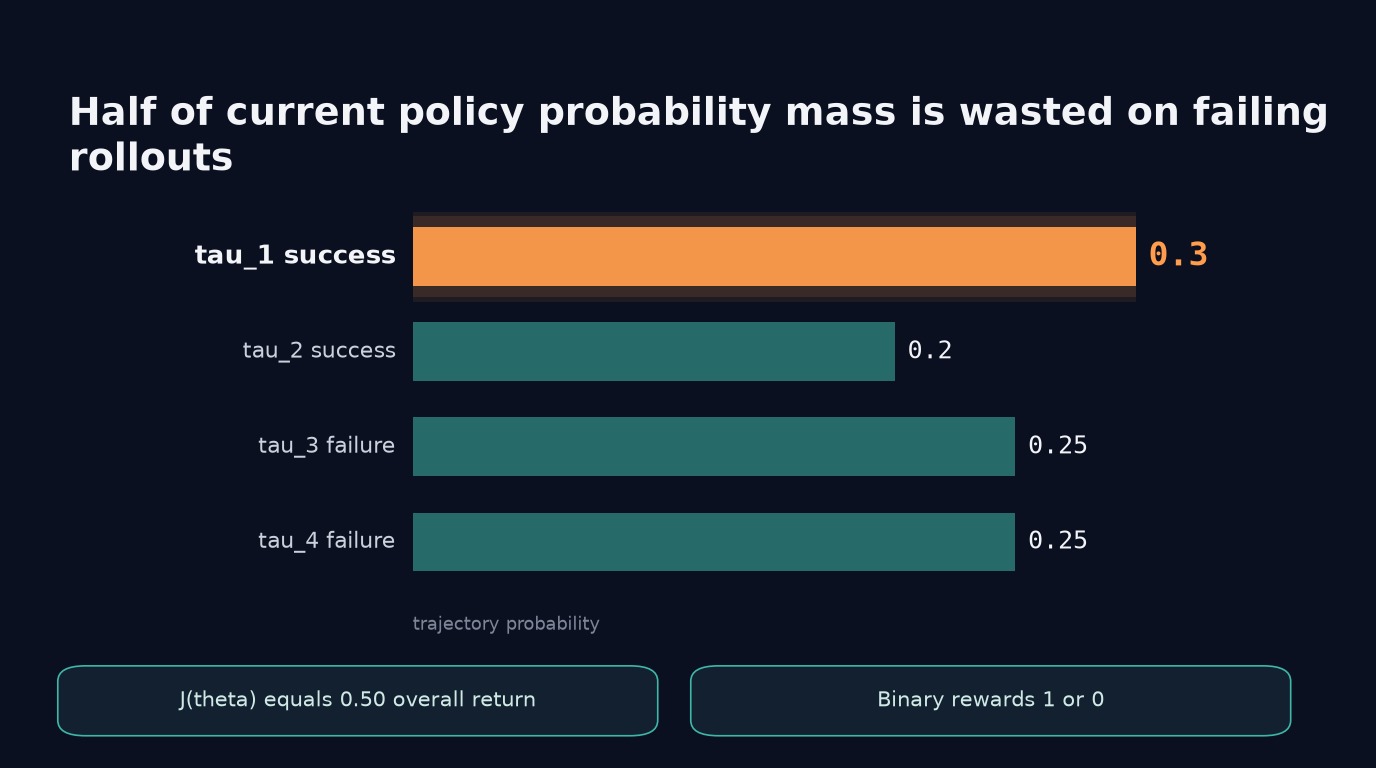
Fig 10. Policy updates shift probability mass from failing trajectory traces toward high-reward episode rollouts.
4. Reinforced Self-Training (ReST)
In short
– ReST alternates rollout generation, reward filtering, and supervised fine-tuning on successes.
– Verified rewards discard failing traces so cross-entropy trains only on successful actions.
– Cold starts and curricula supply early successes when initial policies fail completely.
4.1 The Grow, Improve, and Repeat Loop
Expert iteration modifies supervised fine-tuning (SFT) [Training an agent to imitate a given task demonstration by copying demonstrated actions and maximizing their sequence probability.] through self-generated rollouts.
- Grow: sample trajectories from the current policy parameters and compute their rewards.
- Improve: filter traces by reward, augment high-reward datasets, and fine-tune the policy.
- Repeat: sample fresh trajectories using updated weights and continue fine-tuning the pool.
| Method | Rollout source | Data filtering | Training loss |
|---|---|---|---|
| Self-distillation | Current policy | Keeps all generations | Supervised imitation |
| ReST | Current policy | Keeps verified rewards | Supervised imitation |
- Gulcehre et al.: introduced reinforced self-training (ReST) [An expert iteration loop that generates candidate rollouts, filters them with reward checks, and fine-tunes the policy on the successful traces.].
- Singh et al.: explored the framework as ReST-EM for expectation-maximization policy updates.
- Expectation maximization analogy: Fried notes alternating sampling and updates mirrors the standard EM algorithm.
- Reward filtering: reward checks remove failing rollouts rather than copying arbitrary outputs indiscriminately.
- Dataset growth: newly discovered successful traces continuously enlarge the supervised training buffer.
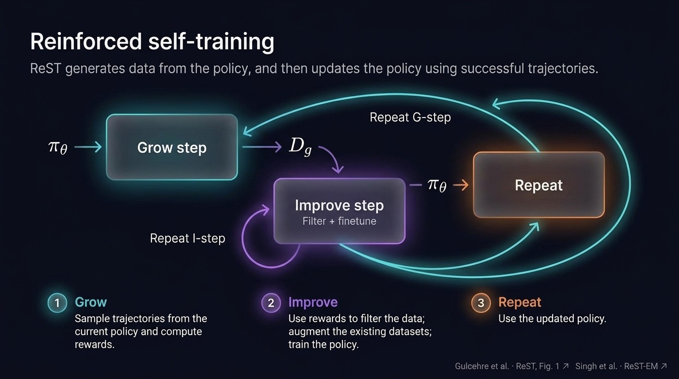
Fig 11. ReST alternates trajectory generation, reward filtering, and supervised policy updates.
Filtering prevents the policy from reinforcing its own mistakes. Supervised updates then stabilize around verified good behaviors.
4.2 Filtering High-Reward Trajectories with SFT Loss
The agent filters candidate trajectories by reward before minimizing cross-entropy on successful actions.
The environment hides a secret integer between 1 and 16, which is unknown to the agent.
- ( R = 1 ) for ( \tau_1 ): guesses 8, 12, 10, hits 11, receives reward 1, and stays.
- ( R = 1 ) for ( \tau_2 ): guesses 4, 8, 12, hits 11, receives reward 1, and stays.
- ( R = 0 ) for ( \tau_3 ): guesses 16, 8, 9, hits 10, times out, and drops.
- ( R = 0 ) for ( \tau_4 ): guesses 1, 2, 3, hits 4, times out, and drops.
- Binary filtering rule: keeps trajectory [A complete sequential rollout recording all observations, agent actions, and intermediate rewards across an episode.] instances scoring 1.
[
\mathcal{L}{\text{ReST}} = – \sum{\tau : R(\tau)=1} \sum_t \log \pi_\theta(a_t \mid h_t)
]
- Action likelihoods: ( a_t ) denotes the action at time ( t ) given conditioning history ( h_t ).
- Cross-entropy objective: standard negative log-likelihood applies exclusively across successful trajectories.
- No policy gradients: shares reward-driven goals with reinforcement learning without full optimization machinery.
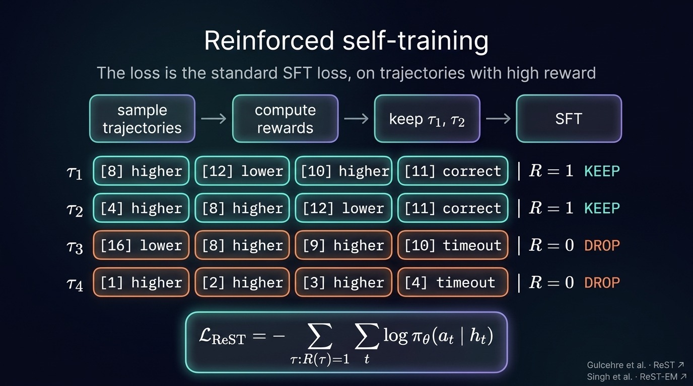
Fig 12. Standard cross-entropy loss trains the model only on traces exceeding the reward threshold.
Dropping failed traces prevents destructive policy drift during training. The objective concentrates probability mass purely on verified sequences.
4.3 Scaffolding Exploration Under Sparse Rewards
Untuned models need exploratory scaffolding when initial policies cannot sample any rewarding rollouts.
- Zero-reward collapse: unguided policies fail on hard tasks and collect zero winning rollouts.
- Cold start traces: human demonstrations or synthetic traces establish early competence before self-training.
- DeepSeek-R1 reasoning traces: pre-trains reasoning behaviors before RL or ReST iterations commence.
- Progressive curriculum: starts on narrow search intervals before tackling the full 1-to-16 range.
- Intermediate shaping rewards: rewards precursor steps like inspecting code repositories before attempting bug fixes.
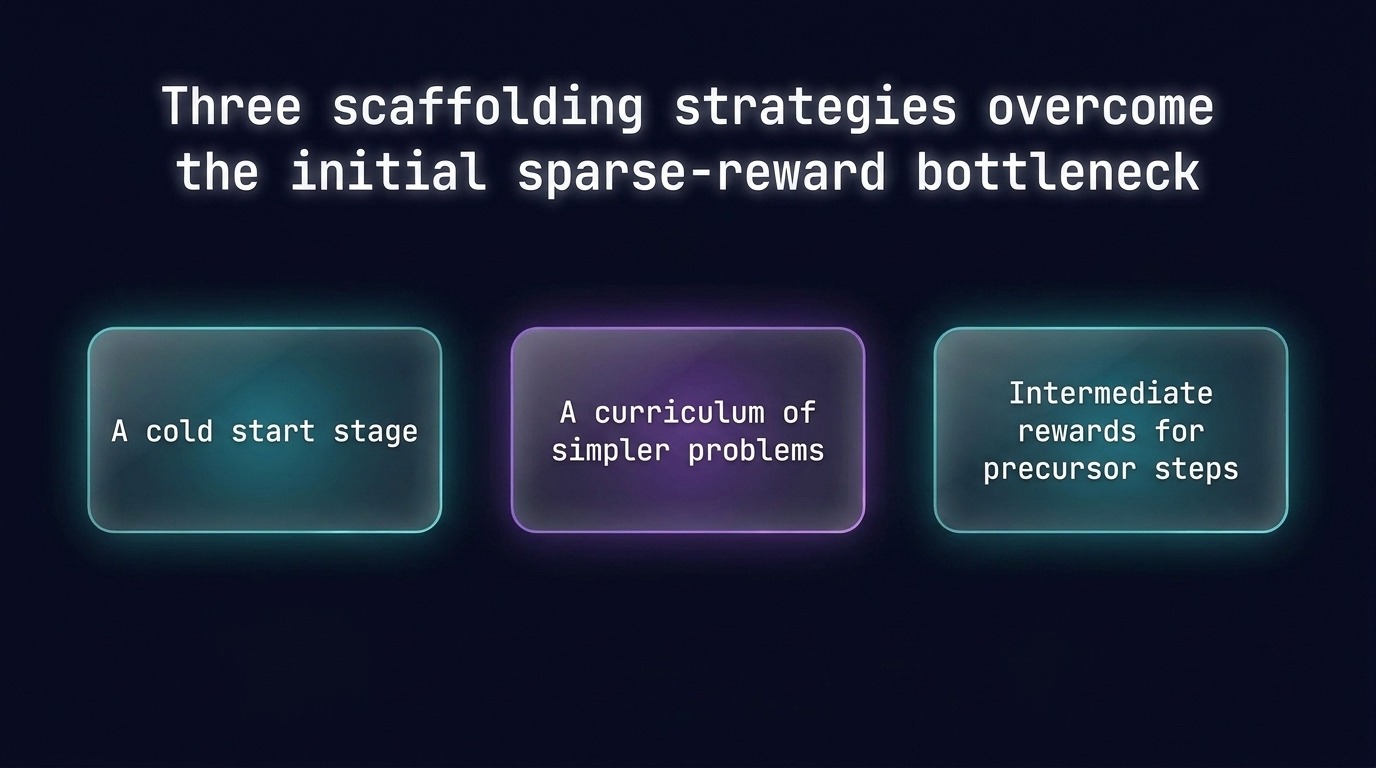
Fig 13. Demonstrations, structured curricula, and intermediate rewards prevent self-training collapse under sparse rewards.
Scaffolding guarantees that early policy rollouts actually encounter rewards. Without positive examples, expert iteration cannot generate training targets.
5. Deriving the Policy Gradient: REINFORCE
In short
– Standard backpropagation fails because discrete sampling and external environments are non-differentiable black boxes.
– The log-derivative trick converts intractable trajectory sums into expectations over sampled on-policy rollouts.
– Environment transition probabilities cancel out, leaving log probabilities of policy actions.
5.1 Limits of standard backpropagation
Direct backpropagation breaks down whenever neural policies interact with discrete external environments.
- 0 derivative almost everywhere: Sampling discrete actions produces piecewise-constant outputs with zero gradients with respect to parameters.
- Non-differentiable environments: Compilers, code execution sandboxes, and game engines cannot compute mathematical derivatives.
- Scalar terminal rewards: Trajectory outcomes yield single evaluation scores only after complete rollout execution finishes.
- 1 to 16 search: If the hidden secret integer is 7, guessing 6 gives zero gradient feedback.
| Optimization attribute | Supervised learning | Interactive reinforcement learning |
|---|---|---|
| Action space | Continuous probabilities | Sampled discrete tokens |
| Environment | Differentiable loss function | Non-differentiable transition dynamics |
| Reward signal | Per-token target labels | Delayed trajectory-level scalar returns |
Backpropagation requires continuous calculation chains connecting outcomes to parameters. Discrete action selection severs this gradient pipeline entirely.
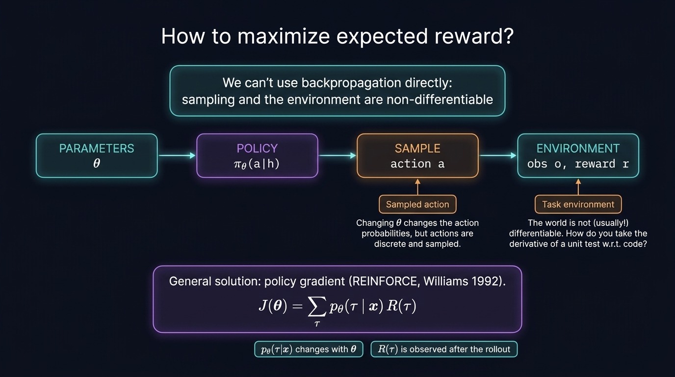
Fig 14. Interactive environments break chain rule differentiation across discrete actions and black-box transitions.
5.2 The five derivation steps
Williams formulated REINFORCE [A foundational policy gradient algorithm that uses sample rollouts and log-probability gradients to maximize expected rewards.] in 1992 using five mathematical transformation steps.
- Express expected reward: Define the objective function (J(\theta)) as an explicit expectation of rewards over all possible trajectories [A complete sequential rollout recording all observations, agent actions, and intermediate rewards across an episode.] (\tau):
[J(\theta) = \mathbb{E}{\tau \sim p{\theta}(\cdot \mid x)} [R(\tau)] = \sum_{\tau} p_{\theta}(\tau \mid x) R(\tau)] - Push gradient inside: Distribute the gradient operator across the summation over trajectories:
[\nabla_{\theta} J(\theta) = \sum_{\tau} \nabla_{\theta} p_{\theta}(\tau \mid x) R(\tau)] - Insert score ratio: Multiply and divide each term by the trajectory probability (p_{\theta}(\tau \mid x)):
[\nabla_{\theta} J(\theta) = \sum_{\tau} p_{\theta}(\tau \mid x) R(\tau) \frac{\nabla_{\theta} p_{\theta}(\tau \mid x)}{p_{\theta}(\tau \mid x)}] - Apply log-derivative trick: Substitute the calculus identity (\frac{\nabla_{\theta} p_{\theta}(\tau \mid x)}{p_{\theta}(\tau \mid x)} = \nabla_{\theta} \log p_{\theta}(\tau \mid x)) using the log-derivative trick [A mathematical substitution that replaces the gradient of a probability divided by that probability with the gradient of its log probability.]:
[\nabla_{\theta} J(\theta) = \sum_{\tau} p_{\theta}(\tau \mid x) R(\tau) \nabla_{\theta} \log p_{\theta}(\tau \mid x)] - Re-express as expectation: Fold the trajectory probability sum back into an expectation over policy-generated rollouts:
[\nabla_{\theta} J(\theta) = \mathbb{E}{\tau \sim p{\theta}(\cdot \mid x)} \left[ R(\tau) \nabla_{\theta} \log p_{\theta}(\tau \mid x) \right]]
The log-derivative transformation converts an intractable complete sum into a tractable expectation. This enables direct Monte Carlo sampling from the current policy.
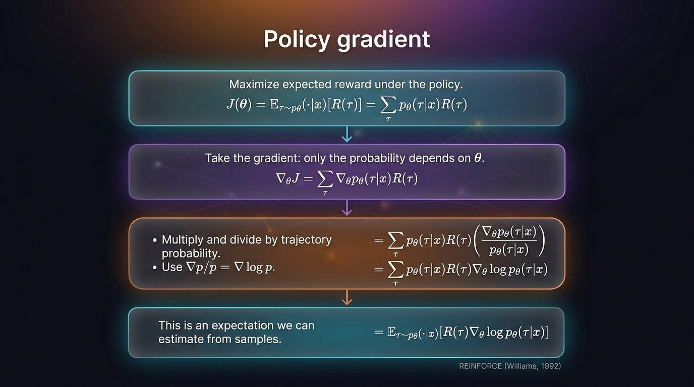
Fig 15. The log-derivative substitution transforms trajectory gradient sums into expectations of log probabilities.
5.3 Core components of REINFORCE
Evaluating empirical policy gradients requires three distinct operational inputs gathered during execution.
- 1 sampled rollout: Agents sample trajectory (\tau \sim p_{\theta}(\cdot \mid x)) on-policy [Sampling interaction rollouts directly from the agent’s current active policy during training rather than from pre-recorded datasets.] using current network weights.
- Scalar trajectory reward: Environment evaluates completed rollout to produce terminal feedback metric (R(\tau)).
- Summed action scores: Backward pass accumulates log-probability gradients (\nabla_{\theta} \log \pi_{\theta}(a_t \mid h_t)) across time steps.
- Unbiased sample estimator: Single-rollout gradient estimate equals (\widehat{\nabla_{\theta} J} = R(\tau) \sum_{t} \nabla_{\theta} \log \pi_{\theta}(a_t \mid h_t)).
- 1 to 16 feedback: Binary reward returns 1.0 on a correct guess and 0.0 otherwise.
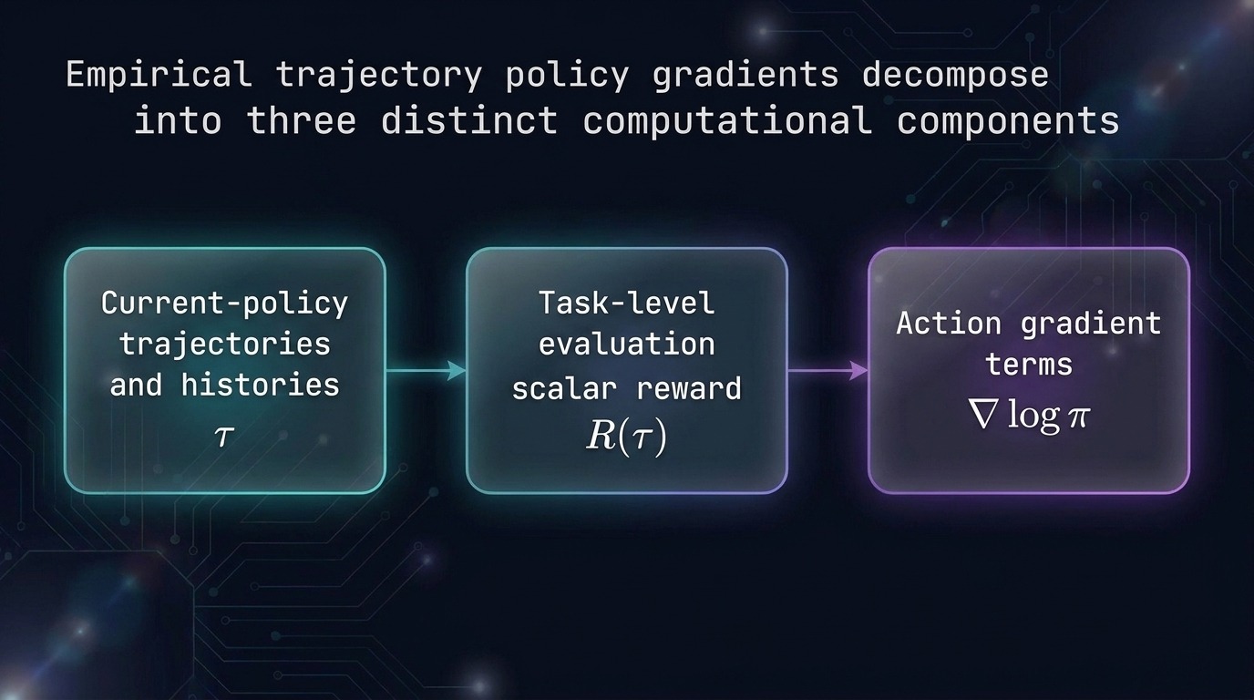
Fig 16. Empirical policy gradient estimation combines on-policy rollouts, trajectory rewards, and action log-probability gradients.
Sampling replaces exhaustive summation across astronomical trajectory search spaces. Empirical averages over sampled rollouts provide unbiased estimates of the true gradient.
5.4 Environment dynamics cancellation
Dynamics cancellation [The theoretical property where non-differentiable environment transitions drop out of the policy gradient because they do not depend on policy parameters.] eliminates unknown environment transition probabilities from optimization equations.
- Trajectory factorization: Full probability (p_{\theta}(\tau \mid x)) factorizes into initial context, policy actions, and POMDP environment transitions:
[\log p_{\theta}(\tau \mid x) = \sum_t \log \pi_{\theta}(a_t \mid h_t) + \sum_t \log P(o_{t+1}, r_{t+1} \mid h_t, a_t, x)] - 0 environment derivative: External environment transitions (P(o_{t+1}, r_{t+1} \mid h_t, a_t, x)) do not depend on policy parameters (\theta):
[\nabla_{\theta} \log P(o_{t+1}, r_{t+1} \mid h_t, a_t, x) = 0] - Clean gradient reduction: Trajectory score reduces strictly to the policy action components:
[\nabla_{\theta} \log p_{\theta}(\tau \mid x) = \sum_{t} \nabla_{\theta} \log \pi_{\theta}(a_t \mid h_t)]
Environment transition mechanics remain completely independent of model parameters. Their derivatives evaluate to zero, allowing model optimization without environment models.
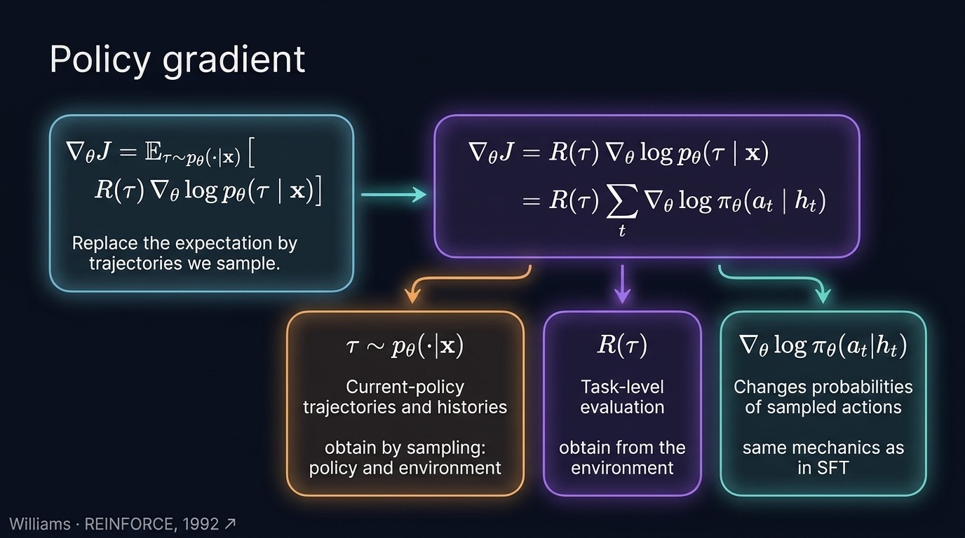
Fig 17. Non-differentiable environment transitions vanish from the gradient, leaving only parameter-dependent policy actions.
5.5 Token-level policy gradient mechanics
Language model agents treat generated text sequences as multi-token compound actions.
- Token decomposition: Action step (a_t) decomposes into sequential tokens ((y_1, y_2, \dots, y_K)).
- Summed token log-probabilities: Multi-token action log probability equals the sum of constituent token log probabilities:
[\log \pi_{\theta}(a_t \mid h_t) = \sum_{k=1}^K \log \pi_{\theta}(y_k \mid h_t, y_{<k})] - Token masking application: Apply token masking [Setting binary indicator flags to separate model-generated action tokens (which receive loss gradients) from context and environment prompt tokens.] to zero out prompt gradients.
- 1 to 16 masking: Mask prompt tokens describing the guessing game, computing gradients solely on guessed digits.
- Cross-entropy reuse: Log-derivative gradients share the identical backward-pass computation graphs used in cross-entropy training.
Autoregressive factorization preserves the mathematical validity of policy gradients across sequences. Language models optimize generated tokens without altering external context representations.
5.6 REINFORCE versus supervised fine-tuning
Comparing REINFORCE to supervised fine-tuning (SFT) [Training an agent to imitate a given task demonstration by copying demonstrated actions and maximizing their sequence probability.] highlights operational differences.
- Objective target: SFT maximizes demonstration token probabilities; REINFORCE maximizes expected cumulative environment return.
- Data source: SFT uses static offline trajectories; REINFORCE samples rollouts dynamically on-policy.
- Weighting mechanism: SFT weights demonstrations equally; REINFORCE scales action log probabilities by scalar reward (R(\tau)).
- Failure recovery: REINFORCE avoids exposure bias [A training flaw where an agent exposed only to pristine demonstrations cannot recover when it makes an error during autoregressive generation.] by letting the agent encounter and correct errors.
| Training paradigm | Data distribution | Optimization objective | Failure consequence |
|---|---|---|---|
| SFT | Offline demonstrations | Token sequence log-likelihood | Error accumulation and compounding |
| REINFORCE | Online policy rollouts | Expected trajectory returns | High gradient estimation variance |
SFT forces exact imitation of fixed demonstration tokens. REINFORCE optimizes task success directly, allowing multiple distinct paths to reward.
6. Scaling and Masking SFT Loss
In short
– Policy gradients scale standard supervised fine-tuning loss using total episode trajectory rewards.
– Token masking isolates generated model actions from environment observations and prompts.
– Binary rewards make online policy gradients algebraically equivalent to offline filtered self-training.
6.1 Token Masking in Agent Sequences
Token masking (setting binary indicator flags to separate model-generated action tokens from context and environment prompt tokens) assigns binary flags across rollout turns.
- 0 for context tokens: user instructions, tool outputs, and environment observations receive zero gradient weight.
- 1 for action tokens: generated completions and end-of-turn delimiter tokens receive active loss gradients.
- 1 to 16 search space: the environment hides a secret integer between 1 and 16, which is unknown to the agent.
guess(8)generation: the agent outputs candidate guesses and turn boundaries as action tokens.higherobservation: the environment returns interactive hints marked as non-differentiable context tokens.
<|im_start|>user ↵ Find·the·number·in·1–16. ↵ <|im_end|> ↵ <|im_start|>assistant ↵
guess(8) ↵ <|im_end|> ↵ <|im_start|>tool ↵ higher ↵ <|im_end|> ↵
<|im_start|>assistant ↵ guess(12) ↵ <|im_end|> ↵ … ↵ <|im_start|>assistant ↵
guess(11) ↵ <|im_end|>
Masking context prevents the model from updating parameters to predict external environment responses. Gradients apply strictly to choices the policy directly controls.
6.2 Reward-Weighted Cross-Entropy Loss
Supervised fine-tuning (SFT) (training an agent to imitate a given task demonstration by copying demonstrated actions and maximizing their sequence probability) adapts directly into a policy gradient objective.
- Objective formulation: the loss sums log probabilities over active tokens and scales by reward.
- Token selection: binary indicator $m_t = 1$ filters generation steps inside the sequence.
- Reward multiplier: one scalar return $R(\tau)$ scales the entire trajectory (a complete sequential rollout recording all observations, agent actions, and intermediate rewards across an episode).
- Direct differentiation: parameter gradients pass through the summation directly into action log probabilities.
- Implementation routine: run standard cross-entropy, apply token masks, multiply by reward, and backpropagate.
[\mathcal{L}{\text{PG}} = – R(\tau) \sum{t: m_t = 1} \log \pi_\theta(u_t \mid u_{<t})]
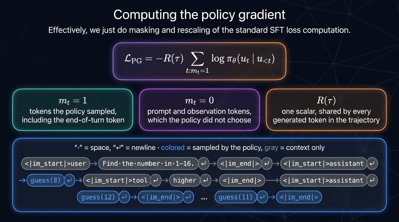
Fig 18. Standard cross-entropy loss transforms into policy gradients through token masking and reward scaling.
Standard loss functions require only minimal engineering changes to optimize language agent trajectories. Masking and multiplication reuse optimized deep learning training pipelines.
6.3 Execution Mechanics: REINFORCE Versus ReST
REINFORCE (a foundational policy gradient algorithm that uses sample rollouts and log-probability gradients to maximize expected rewards) contrasts with iterative dataset filtering.
| Dimension | REINFORCE | ReST |
|---|---|---|
| Sampling mode | On-policy (sampling directly from current policy) | Offline iteration cycles |
| Batch size | 1 rollout per instance | Large filtered rollout pools |
| Loss weighting | Continuous or binary scalar reward | Unweighted positive examples |
| Update cadence | Immediate online parameter updates | Multi-epoch offline fine-tuning |
- Trajectory sampling: agents draw candidate paths directly from current network weights.
- 1 trajectory per instance: basic REINFORCE samples a single attempt per prompt instance.
- Multiple candidate rollouts: group relative policy optimization extends the baseline by comparing multiple paths.
- Data retention: REINFORCE discards sampled episodes immediately following single gradient steps.
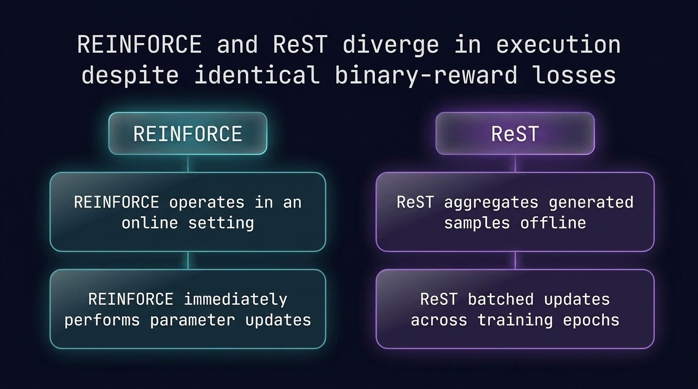
Fig 19. Online policy updates discard fresh rollouts immediately while offline methods train across epochs.
Online collection ensures gradient updates reflect current policy probabilities without distribution shift. Offline buffers trade freshness for compute efficiency across multiple training epochs.
6.4 Binary Rewards and Equivalence Proof
Binary reward functions collapse online policy gradients into supervised imitation of successful traces.
- Assign binary success evaluations $R(\tau_i) \in {0, 1}$ to finished trajectories.
- Evaluate trajectory outcomes against ground-truth unit tests or environment goals.
- Eliminate zero-reward rollouts completely from the objective summation.
- Convert non-zero terms into standard unweighted supervised fine-tuning loss.
- 0 reward elimination: failing attempts drop out because multiplying by zero cancels the loss.
- 1 reward retention: successful trajectories remain inside the objective with unit scale.
- ReST reduction: Reinforced self-training (ReST) (an expert iteration loop that generates candidate rollouts, filters them with reward checks, and fine-tunes the policy on the successful traces) matches this filtered loss.
- Mathematical identity: masked cross-entropy on passing runs produces the identical gradient.
[- \sum_i R(\tau_i) \sum_t \log \pi_\theta(a_{i,t} \mid h_{i,t}) = – \sum_{i : R(\tau_i) = 1} \sum_t \log \pi_\theta(a_{i,t} \mid h_{i,t})]
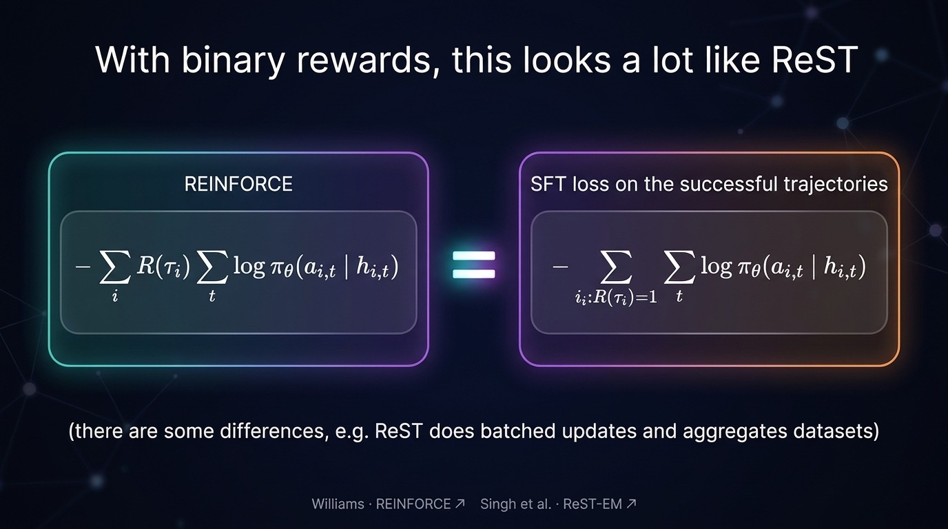
Fig 20. Binary reinforcement learning simplifies algebraically into supervised imitation over passing rollouts.
Zero rewards cancel bad rollouts, leaving only correct solutions in the gradient sum. Algorithmic differences narrow down to data collection schedules rather than loss definitions.
7. Summary
- SFT limitations: Imitating demonstrations penalizes valid alternative paths, ignores failure signals, and induces brittle exposure bias.
- Interactive optimization: POMDP formulations optimize expected trajectory return, shifting model probability mass toward successful, reward-earning rollouts.
- Reinforced self-training: ReST filters self-generated rollouts with verified reward checks, updating policy weights strictly on successful traces.
- REINFORCE derivation: The log-derivative trick eliminates unknown environment transition dynamics, enabling direct gradient estimation from sampled rollouts.
- Loss implementation: Masking context tokens and scaling cross-entropy by binary rewards makes REINFORCE algebraically equivalent to ReST.
Reinforcement learning replaces fixed demonstrations with interactive trial-and-error optimization, enabling policies to directly maximize expected task rewards.
Source
Lecture: Reinforcement Learning Basics by Daniel Fried, Carnegie Mellon University.
Course: CMU 11-768 AI Agents (Fall 2026), Lecture 9, first half.
Video: YouTube · Slides: PDF · Course page: cmu-agents.com
Further reading referenced in the lecture:
- Adapted from Sean Welleck · RL Fundamentals
- Gulcehre et al. · ReST, Fig. 1
- Singh et al. · ReST-EM
- REINFORCE (Williams, 1992)
dataHacker.rs — LLM_log #038: Policy Gradients — From Imitation to REINFORCE. By Vladimir Matic.