#000 Linear Algebra for Machine Learning
Highlights: Linear algebra is a branch of mathematics related to linear equations, linear functions and their representations through matrices and vector spaces. Basically, it is the science of numbers which empowers diverse Data Science algorithms and applications. To fully comprehend machine learning, linear algebra fundamentals are the essential prerequisite.
In this post, you will discover what exactly linear algebra is and what are the main applications in the machine learning.
Tutorial Overview:
You will learn:
- Linear Algebra for Machine Learning basics
- Linear Algebra examples
- Linear Algebra in the field of Statistics
- Matrices and images
- Matrices, Graphs and Recommender systems
1. Linear Algebra for Machine Learning basics
Why do you need to learn Linear algebra?
Linear algebra is a foundation of machine learning. Before you start to study machine learning, you need to get better knowledge and understanding of this field. If you are a fan and a practitioner of machine learning, this post will help you to realize where linear algebra is applied to and you can benefit from these insights.
Vectors, Matrices, and Tensors
In machine learning, the majority of data is most often represented as vectors, matrices or tensors. Therefore, the machine learning heavily relies on the linear algebra.
- A vector is a 1D array. For instance, a point in space can be defined as a vector of three coordinates (x, y, z). Usually, it is defined in such a way that it has both the magnitude and the direction.
- A matrix is a two-dimensional array of numbers, that has a fixed number of rows and columns. It contains a number at the intersection of each row and each column. A matrix is usually denoted by square brackets [].
- A tensor is a generalization of vectors and matrices. For instance, a tensor of dimension one is a vector. In addition, we can also have a tensor of two dimensions which is a matrix. Then, we can have a three-dimensional tensor such as the image with RGB colors. This continues to expand to four-dimensional tensors and so on.

Reading research papers and studying algorithms can be pretty hard without knowing some basic terms. Almost every algorithm is described using the vector and matrix notation. Therefore, we will start with some basic terms that we use to describe matrices:

In addition, one term that is often used is a trace. The trace is the sum of all the diagonal elements of a square matrix.
2. Linear Algebra examples
Next thing that we will talk about is how to add matrices, how to multiply them by scalars, and how to multiply matrices. It is illustrated below as a simple refresher:
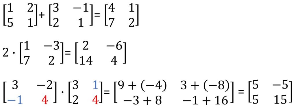
Here is how it works. We need to sum up the corresponding entries and we have our answer, it is really simple. Next, to multiply a matrix by a single number (scalar), we need to multiply every entry by that value. When it comes to matrix multiplication, thins are a little different, we do this row by column element-wise multiplication.
Now, let’s see what happens when we multiply a vector by a matrix. For example, a vector that starts at the origin and ends at (1, 1) can be written in a matrix form. The \(x \) component is at the top and \(y \) component is at the bottom.

When we multiply an “in” vector by a \(2\times 2 \) matrix, we get a new vector “out”. In our example, it is (1, 3) output vector.
There are some special matrices that transform our input vectors in an interesting way. Let’ have a look at how this matrix rotates a vector for 90 degrees in a counterclockwise direction.

In addition, some matrices are capable to scale the input vector:

Any vector on the same line as our input vector, will be mapped to a vector on the same line as the corresponding output vector. These examples of vector processing we also call linear transformations.
The linear transformations are the reason why we call the first in-depth class on matrices: Linear Algebra. We are going to revisit these transformations later, but now it is the right time to pay attention to the following input vector (2,1).
You will notice that it is only scaled when it is multiplied with a \(2×2\) matrix, and it doesn’t rotate at all. This would happen to any vector on that same line. Any vector that is only scaled by a matrix is called an eigenvector of that matrix. And how much the vector is scaled we call the eigenvalue. In our case the eigenvalue is 2 since the original vector doubled its length.

Last but not least, here is the first application of matrices that we typically learn in school. It is how to solve systems of linear equations using matrices.

The coefficients can go into one matrix and the variables (x,y) go into another one. Then, we also have one matrix to store the output (1,3). Using the rules of the matrix multiplication we can see that the first and the second equations are exactly the same.
So, the question is: what is the input vector that our matrix will map to the output vector (1, 3)?

It is interesting to illustrate the solution of this equation graphically.

In order to solve this, we can introduce the concept of an inverse matrix. So, if we know an inverse matrix and multiply it with our known output vector (1,3), we will get our result.

When we are applying an inverse matrix, that process is known as going backwards. When the desired output is the multiplied with an inverse matrix, then we get our solution: \(x= 1 \) and \(y= 1 \).
3. Linear Algebra and Statistics
Linear algebra has left its fingerprint on many related fields of mathematics, including statistics. Data analysis and statistics are another essential field of mathematics that support machine learning. Modern statistics uses both the notation and tools of linear algebra to describe techniques of statistical methods. Examples range from vectors for the mean and variances of data, to covariance matrices that describe the relationships between multivariate Gaussian variables. The results of some collaborations between linear algebra and statistics are directly applicable in machine learning methods. For instance, the Principal Component Analysis (PCA) is used for a dimensionality reduction.
Example. So, let’s say that we have a system that continuously evolves over time. For example, let’s say there’s a Coronavirus (COVID-19) outbreak at the local high school and the place is quarantined, so that no one can go in or out.
But the virus is spreading inside!

So, we have healthy and infected people in the school and no one is coming in or out, so the overall population remains the same. Now, let’s say that every day 20% of healthy people will get sick. There is a cure for the disease, however, it’s not always guaranteed to work.

So, we’ll say that every day 10% of the infected people will get healed. At this moment, if there are 150 infected and 150 healthy humans the question is what is going to happen in the long run. Now, we are going to assume that the changes happen in discrete intervals at the daily level. So, let’s see what happens in the first day. For the healthy humans (150), 80% of them are going to stay healthy and will not be infected. We also have to add the 10% of the 150 infected that become cured. This leaves us with a 135 healthy people after the first day. For the new total of infected we would take the 20% of humans that got infected plus the 90% of the 150 infected that are not cured. This gives us a total of 165 infected.

So, this is after the first day. However, we want to know what happens after a long time so we got to keep going with this procedure. After another day we write the same percentages, except now, the number of healthy persons is 135 instead of 150. For the infected we got 165 instead of 150. This now puts 125 for the healthy and 175 for the infected after two days.
So, it looks like more people are getting infected. Will this trend continue? Well, let’s see. What we have here is some linear equation that can be represented as a matrix of those percentages which don’t change. This is multiplied by the inputs h (healthy) and i (infected) at any given time.

This is called a Markov matrix, its column sum to 1 and it doesn’t have negative values. We have already explained what can happen to a vector multiplied by a matrix. This matrix is going to scale and rotate the input vector. The first input was (150, 150), and that was the initial healthy and infected population. The following day, the vector moved to (135, 165). And, we have to keep going and apply another transformation sending it to (125, 175). That was the populations that we found after 2 days.
So, as we keep applying these multiplications the real question is where does this vector go?
The solution will actually converge to some equilibrium point. And this point can be determined with the use of eigenvectors.
This kind of math could be used to analyze how a virus will spread throughout a population for example. One similar application of this is the Google page rank algorithm. It involves Markov matrices and ranks websites by treating outgoing links as the probabilities of transitions from one site to another.
Matrix factorization
In order to interpret advanced matrix operations, you must understand matrix factorization. It is very important to know what kind of matrix factorization algorithms do exist and when they should be applied.
In simple words, we are using a matrix factorization to decompose a matrix. As a result, we get two or more matrices. Next, we can multiply them back together, and we will get the original matrix. The matrix factorization is a key tool in linear algebra and it is widely used as a building block for more sophisticated operations. Furthermore, there is a range of different matrix factorization methods. The most known one is the Singular Value Decomposition (SVD).

Linear Least Squares
After matrix factorization, the next type of problems are linear least-squares problems. This is an approach to fitting a mathematical or statistical model to data. Usually, in such cases we have a set of data points provided by the model that shows a linear relation with the unknown parameters of the model. Linear least-squares problems can be solved efficiently on computers using matrix operations such as matrix factorization. Least squares are most known for its role in the solution to linear regression models, but also plays a wider role in a range of machine learning algorithms.
4. Matrices and images
What is a digital image?
Let’s have a look at what a digital image is. When we look really closely it is just made up of a bunch of pixels each of a single color. A pixel is a small element of a picture. Each pixel represents a color which is a combination of three-color channels: red, green and blue. With a million combination of these colors, we can represent any color and any image.

In computers, images are commonly stored as matrices. To represent a single channel intensity, we will use values from 0-255. So, for one color pixel we need three times 8 bits for a representation. For the grayscale images, on the other hand, we use values from 0-255 to represent gray intensities: 0-black and 255-white. For them, we only need 8 bits or 1 byte of data for storage.
Are you on Instagram?

Well, Instagram is all about images, filters and #nofilters. Let’s have a look what a filter actually does. We are going to mathematically blur this grayscale image shown below. To do this we are going to make a \(3\times 3 \) matrix where every entry is 1/9. This is known as a filter in image processing. Then, we’re going to lay this filter over our image matrix and multiply the individual entries in each square together and then add the results. This is known as a convolution operation.
You can read more about convolution on RGB images here.

This was just one basic example of how we can smooth our image. A bunch of other filters exist and depending on the filter coefficient values they do various cool things. Just to name a few, they can sharpen, blur or smooth images.
5. Matrices, Graphs and Recommender systems
Now, let’s have a look at networks and graph theory. Graphs can represent a lot of things.

We can use graphs to show people that know each other (e.g. FaceBook) or people who are business partners (e.g. LinkedIn). Then, we can discover our common friends or who is the most popular person. And the cool thing is, that graph connections can be represented as matrices!

If you are interested how many mutual friends two people have in our mockup graph it is not a big deal. You can just count them. But, when the networks get more complex, we need mathematical tools to help us identify the key insights. For example, which website should be ranked the highest on the web. How to identify people involved in the 9/11 terrorist attacks? And who was the most critical to the operation and should be prioritized by law enforcement? Such analysis were actually done after 9/11. Thus, we need some mathematical techniques in these cases, when our eyes aren’t powerful enough to see those chaotic connections.

Another application of graphs can be a dating app. Imagine this app only has three women signed up that we will label 1 through 3. Also, there are 3 men labeled 4 through 6 as shown in the graph above. The mutual connections revealed who liked who – mutual right swipe in the app :-). Here, there are no same-sex matches. We see this first woman matched with all three guys. The second woman with 2 and the third with 1. Now, this graph provides a nice visualization for this situation. We will use it to illustrate how we can do the same thing with a \(6×6\) matrix for these 6 people and analyze the hotness and loveliness. Therefore, we’ll say if two people are matched we will signify this with 1 in a matrix and 0 if they are not a match. For instance, let’s have a look at persons 1 and 4. They liked each other so (1,4) element will be 1. In addition, we will do the same for the element (4,1) since these are mutual connections.
Obviously, this matrix will be symmetric.

Then, if two people are not connected (like person 1 and 2), we’ll put a 0. Here, it will be for elements (1,2) and (2,1) in our matrix. We illustrate this below.

OK, we are all narcissists. But, no one matches with themselves, so the diagonal is going to be all 0s and then these would be the rest of the connections. So if you want to know whether person 5 and 2 are connected by the table just go to column 5 and row 2 or vice versa and see if there’s a 1 or a 0 there.

Therefore, there are obvious things we can see. Like for person 1 we can look down their column or across the row and find they have three matches in total because of the three 1s. But, instead of considering this as a table, we are going to call it a matrix. When it comes to graphs this is known as an Adjacency matrix.

It tells us how many paths of length 1 exists between any two nodes. So, what does this really mean? We’ll look at column 6 and row 1. We know that this says that those two people are matched. Moreover, it also means that there is one path of length one that exists between them. Those are saying the same thing. If we put a dot at person 1 and can only traverse one edge well there’s one way to get to person 6. That’s what this one represents.

On the other hand, there are 0 ways to get from person 1 to person 2 in one edge.

If you start a person 1 there are paths to person 2 but they all have a length of 2 which is not what we were looking for. But now what if we want to see quickly how many mutual matches two people have. Well, if we look at person 1 and 2 this isn’t difficult. We see that there are 2 mutual matches. However, this question of mutual matches is no different than asking how many paths of length 2 exists between person 1 and person 2. Well, we just solved that. The answer is 2 as expected since it’s the same question. Again, if we start at 1 and go to 4 then 2 or 5 then 2. Those two paths mean two mutual connections. The cool thing is that we can find how many of these paths of length 2 exist between any two nodes by just multiplying the adjacency matrix by itself or squaring it.

We see for person 1 and 2 there are 2 mutual connections so that checks out. Then if you look at the graph for person 2 and 3, they have no mutual connections. On the matrix this checks out as well from column 3 and row 2 having a 0. However, person 1 and 3 are both connected to 6 and no one else which we can also find in the matrix and you get the idea. Now what would the diagonal mean? Well that’s how many paths of length 2 exists between a person and themselves a.k.a. how many matches they have.

Now if we have a same-sex connection and link one to two let’s say all we have to do is add a 1 to the original matrix in the first column second row and vice versa. When implementing this in the software we just have to make small tweaks to the adjacency matrix and from there squaring or cubing it tells us a lot.
Well, we really do hope that you will find some fun in all these examples! Finally, let’s review some of the most important:
Applications of Linear Algebra

Summary
Well, this was our reeeaaaaly lengthy post about Linear Algebra applications :-). With this motivating examples we hope that you realized the importance of Linear Algebra and that you are ready for a deep dive into the essence of Linear Algebra. Let’s roll!
References:
- Basics of Linear Algebra for Machine Learning. Jason Brownlee.
- The Applications of Matrices | What I wish my teachers told me way earlier. Zach Star.


