CamCal 003 Camera Transformation
Highlights: In this post we will talk about camera calibration technique, and rigid body transformations. You will also see how translation and rotation works.
Tutorial Overview:
1. Intro
In this post, we’re going to talk about extrinsic camera calibration and here is the model that we are going to use.
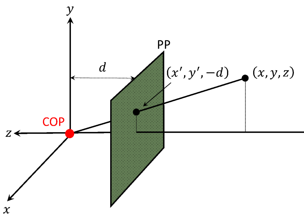
In particular, we had a system where we had a center of projection (COP) that was located at the origin of a three-dimensional camera system. And then we derived from similar triangles the location on the image of the point projected down onto the image plane. And then in order to figure out where the point was going to land on the image, we just eliminated that last coordinate.
Projection equations:
$$ \left ( X,Y,Z \right )\rightarrow \left ( -d\frac{X}{Z},-d\frac{Y}{Z},-d \right ) $$
$$ \left ( {x}’,{y}’ \right )= \left (-d\frac{X}{Z},-d\frac{Y}{Z} \right ) $$
Now we said that this was a bit of an issue because this division by \(Z \) was non-linear. So we introduced this notion of homogeneous coordinates:
Homogeneous image – (2D) coordinates
$$ \left ( x,y \right )\Rightarrow \begin{bmatrix}x\\ y\\ 1\end{bmatrix} $$
Homogeneous scene – (3D) coordinates
$$ \left ( x,y,z \right )\Rightarrow \begin{bmatrix}x\\ y\\ z\\ 1\end{bmatrix} $$
And the idea was, that we were going to be able to convert from homogenous to non-homogenous when we needed them.
Converting from homogenous coordinates:
$$ \begin{bmatrix}x\\ y\\ w\end{bmatrix}\Rightarrow \left ( x/w,y/w \right ) $$
$$ \begin{bmatrix}x\\ y\\ z\\ w\end{bmatrix}\Rightarrow \left ( x/w,y/w,z/w \right ) $$
But before we did that, all of our operations could be done through matrix multiplication. Which, by the way made homogenous coordinates, the whole thing, invariant under scale.
One of the reasons we did this is we said that perspective projection could now be done as matrix multiplication. And by the way, just to make life easier, we are using the absolute value of \(z \), so we don’t have to worry about \(z \) being positive or negative. So, when we do the multiplication, we get this homogeneous coordinate. And when we want to normalize and go to nonhomogeneous, we get the \(\left
$$ \begin{bmatrix}1 & 0 & 0 & 0\\ 0 & 1 & 0 & 0\\ 0 & 0 & 1/f & 0\end{bmatrix}\begin{bmatrix}x\\ y\\ \left | z \right |\\ 1\end{bmatrix}= \begin{bmatrix}x\\ y\\ \left | z/f \right |\end{bmatrix}\Rightarrow \left ( f\frac{x}{\left | z \right |},f\frac{y}{\left | z \right |} \right )\Rightarrow \left ( u,v \right ) $$
But in all of this discussion about projection, we have the notion of a camera’s coordinate system. So we have an origin and a coordinate system. And we said that we put the
2. Geometric camera calibration
This whole thing falls under the labelling of geometric Camera Calibration. In order to be able, for the camera to tell us about things in the world, we need to know the geometric relationship between the camera and the world. Geometric camera calibration is composed of two parts. First, we need to know the relation between the world and the camera. This is a relation between two 3D coordinate systems and is represented by extrinsic parameters. Second, we need to know the process of mapping a 3D world onto a camera plane and these are known as intrinsic parameters. So let’s talk about camera pose or the orientation and location of the camera frame with respect to the world coordinate system.
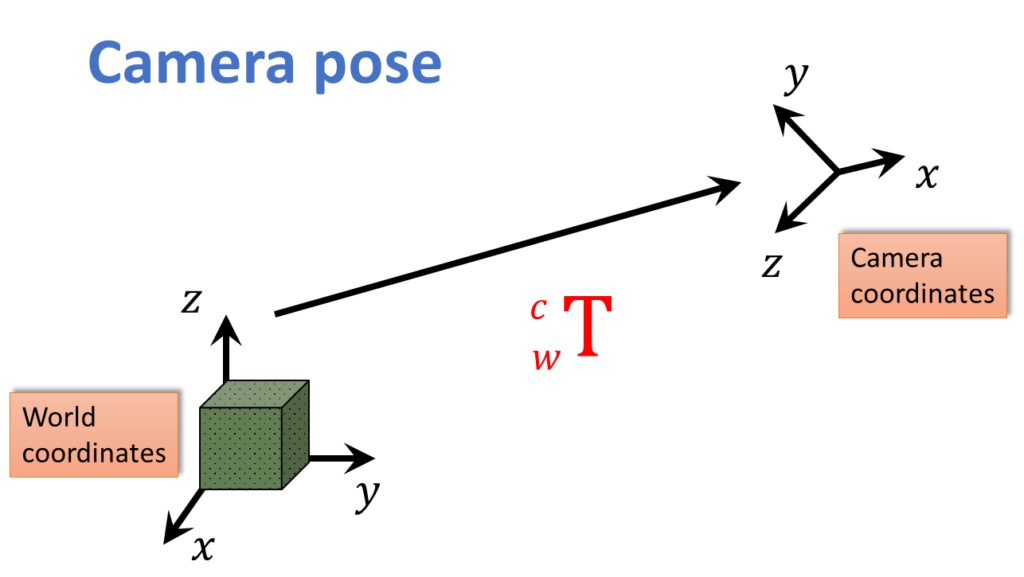
In this diagram, this transform \(T \) is a transform that goes between the world and the camera system. And that is what this \( _{w}^{c}\textrm{T}\) is going to mean. The transformation that we are going to talk about is this going from world coordinates to camera coordinates.
3. Rigid body transformations
Well, you can see, easily think about it this way. Let’s define a rigid body as just a collection of points whose relative positions to each other can’t change.
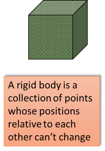
For our demonstration here, we will assume that the rigid body is simply a box.

We can take one point of that box (black dot), say the corner here, and figure out the \(x \), \(y \) and \(z \) location of that box. So, that is three degrees of freedom – dof. Then, we can take some other point on that box (red dot), let’s say the corner, and we can move it around. Now, we can’t change it’s location space arbitrarily because we are holding this point fixed. Essentially, this corner can move around on the sphere. So, this point here can be moved around anywhere on the sphere (red arrow). There is two degrees of freedom of a vector’s direction. So, that is another two degrees of freedom. So, we are up to five. And finally, once we have this vector specified (black arrow), we can rotate, we can spin about that vector. So, the cube here, as indicated by green arrow that is in here, we can rotate it about that diagonal. That is one more degree of freedom. So, that is why there are six degrees of freedom for a rigid body.
4. Notation
The idea here is that superscripts are going to represent what coordinate frame you are in.
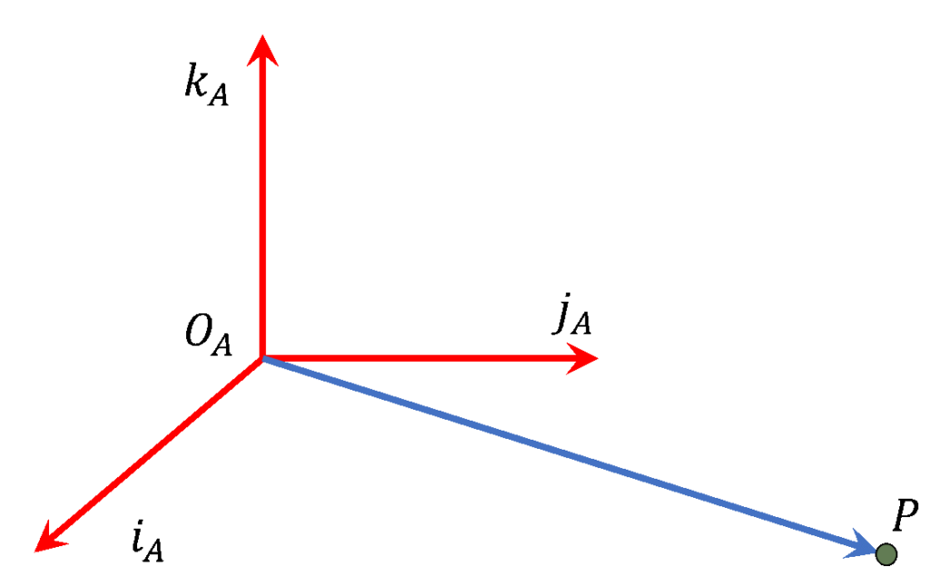
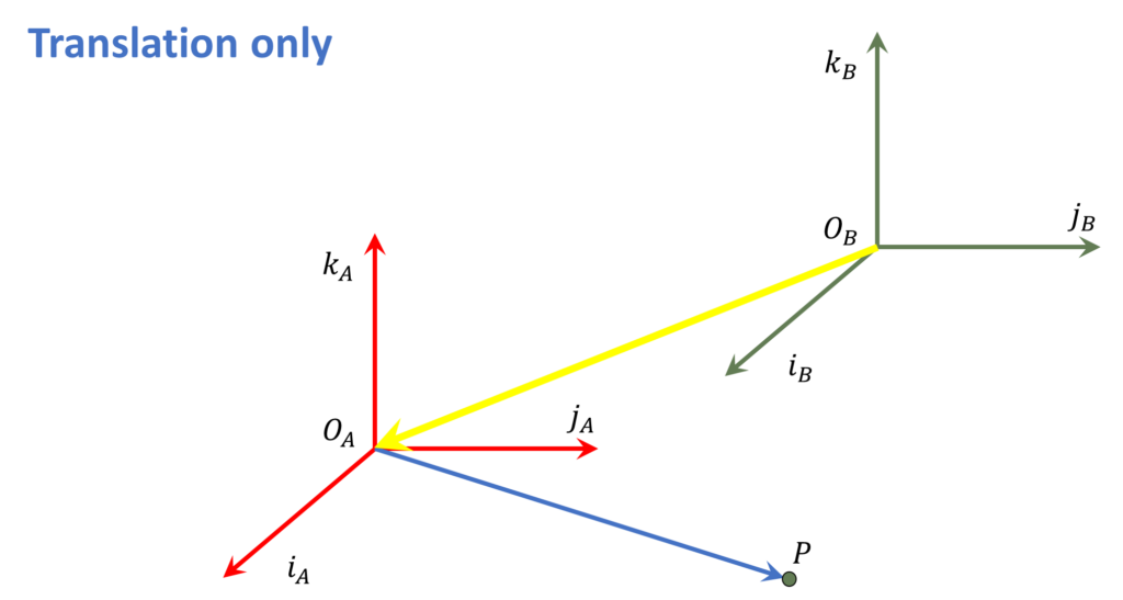
So here we have some point \(P \) and we have got the \(A \) coordinate frame. And the expression of the location of \(_{ }^{A}\textrm{P}\) can be thought of as a variety of ways. We can think of it as the location of \(_{ }^{A}\textrm{x} \), \(_{ }^{A}\textrm{y} \), \(_{ }^{A}\textrm{z} \). But if you remember a little but from your algebra, the right way of thinking about the vector that goes from the origin to \(P \), that is this vector \(\overrightarrow{OP}\), it is got the \(\overrightarrow{i_{A}} \) component of the amount \(_{ }^{A}\textrm{x} \), the \(\overrightarrow{j_{A}} \) component of the amount \(_{ }^{A}\textrm{y} \) and this \(\overrightarrow{k_{A}} \) component of the amount \(_{ }^{A}\textrm{z} \). So, a vector is actually the sum of these three components each scaled by the coefficients, \(_{ }^{A}\textrm{x} \), \(_{ }^{A}\textrm{y} \), and \(_{ }^{A}\textrm{z} \).
$$ { }^{A}\textrm{P}=\begin{bmatrix}_{ }^{A}\textrm{x}\\ _{ }^{A}\textrm{y}\\_{ }^{A}\textrm{z}\end{bmatrix}\Rightarrow \overrightarrow{OP}= \left ( _{ }^{A}\textrm{x}\times \overrightarrow{i_{A}} \right )+\left ( _{ }^{A}\textrm{y}\times \overrightarrow{j_{A}} \right )+\left ( _{ }^{A}\textrm{z}\times \overrightarrow{k_{A}} \right ) $$
Suppose we want to express the location of point \(P\), whose value we might know in coordinate frame \(A \) , but we would like to know where it is in terms of coordinate frame \(B \). Well that is just a translation and it is handled very simply by saying, the location of \(_{ }^{B}\textrm{P} \) is just the location \(_{ }^{A}\textrm{P}\) plus the location of the origin \(_{ }^{B}\textrm{O}_{A}\) frame.
$$ _{ }^{B}\textrm{P} = _{ }^{A}\textrm{P} + _{ }^{B}\textrm{O}_{A} $$
And so that equation just gives us that new offset and this \(_{ }^{B}\textrm{O}_{A}\), that is just a three vector. That is the offset of the origin of \(A \) in the \(B \) frame.
The good news is once again, homogeneous transformations or we should say, homogeneous coordinates are going to come to our rescue. Then, a translation can be expressed as a multiplication. So we have rewritten this equation \(_{ }^{B}\textrm{P}= _{ }^{A}\textrm{P}+_{ }^{B}\textrm{O}_{A}\), as this matrix transformation.
$$ \begin{bmatrix}_{ }^{B}\textrm{P}\\ 1\end{bmatrix}= \begin{bmatrix}I & _{ }^{B}\textrm{O}_{A}\\ 0^{T}& 1 \end{bmatrix}\begin{bmatrix}_{ }^{A}\textrm{P}\\1\end{bmatrix} $$
A couple of things, first of all, that \(I \), that is a \(3\times 3 \) identity matrix, and since \(_{ }^{B}\textrm{O}_{A}\) is a \(3\times 1 \), this is a \(4\times 4 \) matrix. Just to remind you, a translation is commutative.
5. Rotation
Now, what we are showing here are two coordinate frames, \(A \) and \(B \).
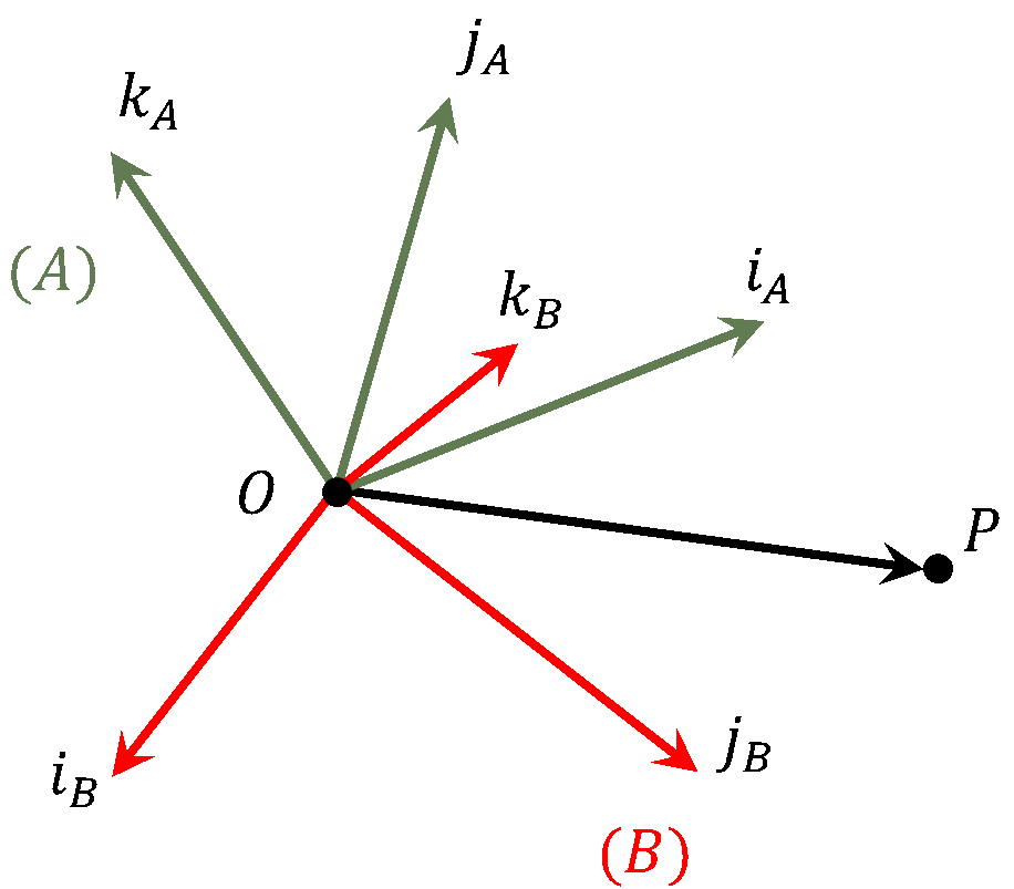
And you will notice that \(A \) has an \(i \) vector, a \(j \) vector and a \(k \) vector. Also \(B \) has an \(i \) vector, a \(j \) vector, and a \(k \) vector. And one of the important things to realize is that this \(P \) value, the vector from the origin can be expressed in two ways. It can be expressed as some components in the \(A \) frame times the \(x, y, z \) components, or some components in the \(B \) frame with the components in the \(x, y, z \) frame. They are the same vector. And what’s key is understanding that there are these basis vectors and we need to know the amount of component that multiplies each of them.
$$ \overrightarrow{OP}= \left ( i_{A}, j_{A}, k_{A} \right )\begin{bmatrix}_{ }^{A}\textrm{x}\\ _{ }^{A}\textrm{y}\\ _{ }^{A}\textrm{z}\end{bmatrix}= \left ( i_{B}, j_{B}, k_{B} \right )\begin{bmatrix}_{ }^{B}\textrm{x}\\ _{ }^{B}\textrm{y}\\ _{ }^{B}\textrm{z}\end{bmatrix} $$
What we need is a relation that combines rotation of a frame from \(A \) to \(B \), and this is how we can express it:
$$ _{ }^{B}\textrm{P}= _{A}^{B}\textrm{R}_{ }^{A}\textrm{P} $$
What this says is given our point described in \(A \), we are going to have a rotation operator that would give us the \(P \) now expressed in the \(B \) frame. And \(_{A}^{B}\textrm{R} \) means describing frame \(A \) in the coordinate system of \(B \). And that means that if you gave us the location of a point in terms of the components of \(A\), this is and it is only a rotation after applying \(R \), we get the components in the frame \(B \).
Summary:
To conclude, here we started our work on camera calibration, and we have covered some basics of rotation. In the next post, we will talk more about how does \(R \) look like and continue working on calibration.