LLM_log #039: Policy Gradient Baselines — From REINFORCE to GRPO

Policy Gradient Baselines — From REINFORCE to GRPO
Highlights: Subtracting a simple 0.5 baseline cuts the gradient’s standard deviation from 0.325 to 0.108 without biasing the update, and GRPO gets its baseline for free from a group of rollouts. In CMU 11-768 AI Agents (Fall 2026), Daniel Fried explains why reinforcement learning for language agents requires relative reward baselines rather than raw trajectory returns. We walk through the mathematical proof of zero-bias baselines, analyze variance reduction in a two-armed bandit simulation, and trace the evolution from PPO to critic-free methods like GRPO and DrGRPO.
- Zero gradient on failure: Standard REINFORCE leaves policy parameters unchanged on zero-reward trajectories, completely preventing error correction on failed attempts.
- Zero baseline bias: Action-independent baselines conditioned strictly on history introduce zero gradient bias because total action probabilities sum to one.
- Bandit variance reduction: Centering binary rewards with a 0.5 baseline reduces gradient estimator standard deviation from 0.325 to 0.108 while maintaining the identical expected update of 0.1875.
- Critic-free GRPO: Group-Relative Policy Optimization eliminates auxiliary value networks by calculating empirical baseline means and standard deviations across rollouts sampled per prompt.
- DrGRPO corrections: DrGRPO removes group standard deviation scaling and replaces variable-length division with a constant budget to prevent task difficulty distortion and verbosity drift.
Tutorial Overview:
- Why Rewards Must Be Relative
- Baselines and the Advantage Function
- A Minimal Two-Armed Bandit Simulation
- Intermediate Rewards: The Reward-to-Go Formulation
- Group-Relative Policy Optimization (GRPO)
- DrGRPO: Fixing Pathologies in Standard GRPO
- Failure Modes, PPO Comparison, and Unification
- Summary
1. Why Rewards Must Be Relative
In short
– Raw trajectory rewards yield zero gradient on failures, completely preventing error correction.
– Baselines convert raw returns into relative advantages to penalize mistakes appropriately.
– Rare failures on easy tasks require strong negative updates against expected returns.
1.1 Limits of raw trajectory rewards
Standard policy gradient methods fail when updates depend purely on unshifted, absolute reward values.
- REINFORCE (a policy gradient algorithm scaling updates by unshifted rewards): leaves parameters unchanged on zero-reward failures.
- $R = 0$ update elimination: produces zero gradient in REINFORCE and ReST, ignoring fatal mistakes.
- $R = 1$ equal upweighting: boosts every intermediate step equally regardless of individual action quality.
- 95% success baseline (a reference value subtracted from rewards): makes rare 5% failures yield massive negative updates.
- Advantage (a metric measuring return relative to expected return): scales policy gradients (parameter updates proportional to advantages) effectively.
| Trajectory | Guesses and feedback | Reward | Policy update |
|---|---|---|---|
| $\tau_1$ (Success) | 8 (higher), 12 (lower), 10 (higher), 11 (correct) | $R = 1$ | Upweights all steps equally |
| $\tau_3$ (Failure) | 16 (lower), 8 (higher), 9 (higher), 10 (timeout) | $R = 0$ | Zero gradient; ignores mistakes |
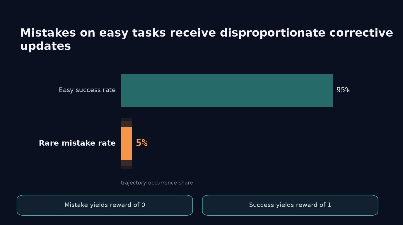
Fig 1. Rare mistakes on easy tasks require strong negative updates against expected baseline rewards.
Shifting rewards creates relative signals so agents learn which specific choices caused failure. Relative scaling ensures gradient steps reflect task difficulty rather than arbitrary reward scales.
2. Baselines and the Advantage Function
In short
– Advantage evaluates whether an action outperforms the policy’s average expected return.
– History-conditioned baselines reduce gradient variance without introducing estimator bias.
– Baseline designs determine core algorithm families including REINFORCE, PPO, and GRPO.
2.1 Formalizing Advantages in Guessing Games
Fried formalizes advantages in a number guessing game where agents discover hidden numbers through sequential guesses.
- Advantage metric: Advantage (A metric measuring how much better a specific action or trajectory is compared to the policy’s average expected return.) evaluates action quality: $A^\pi(h, a) = Q^\pi(h, a) – V^\pi(h)$.
- Action-value definition: $Q^\pi(h, a)$ computes expected return after choosing action $a$ under autoregressive policy $\pi$.
- State-value definition: $V^\pi(h)$ computes expected return when sampling all subsequent actions directly from policy $\pi$.
- Fried’s guessing setup: Guesses 8 (“higher”) and 12 (“lower”) leave target candidates 9, 10, and 11.
- 1 versus ~2/3 return: Optimal policies achieve 1 expected return; random valid policies achieve roughly 2/3 return.
- 10 versus 11 advantage: Guess 10 yields $A > 0$; guess 11 leaves two remaining candidates ($A < 0$).
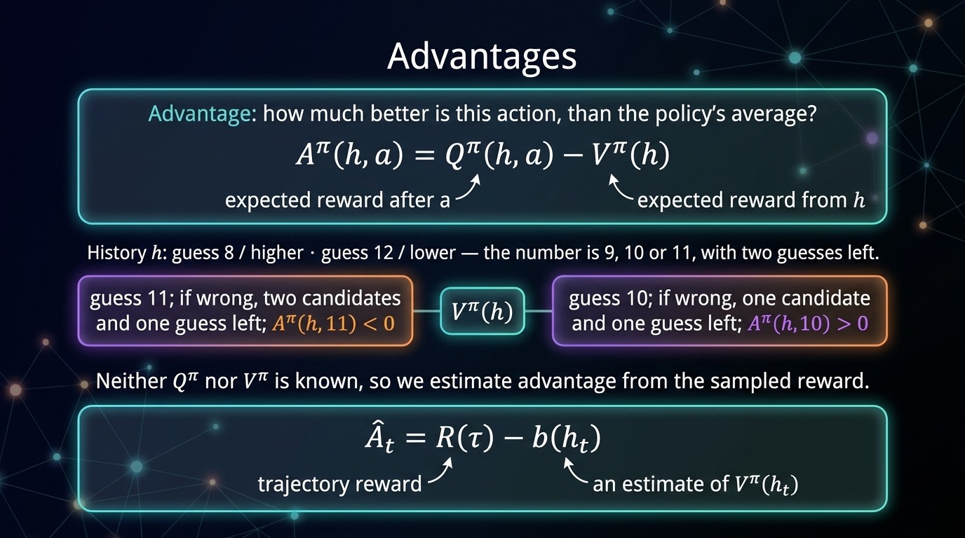
Fig 2. Advantage functions quantify action quality relative to the baseline state value.
Centering action returns around state values highlights genuinely superior choices. It prevents penalizing good actions taken in difficult states.
2.2 Policy Gradients with Baseline Functions
Empirical advantage estimators subtract history-dependent baselines from sampled trajectory rewards to approximate intractable value expectations.
- Empirical advantage formula: Empirical advantage $\hat{A}_t = R(\tau) – b(h_t)$ approximates unobservable theoretical advantages during training.
- Baseline role: Baseline (A reference value subtracted from trajectory rewards to evaluate whether an outcome was better or worse than expected without biasing gradient updates.) approximates state return $V^\pi(h_t)$.
- REINFORCE update: REINFORCE (A basic policy gradient algorithm that scales updates by the raw, unshifted trajectory reward, failing to actively penalize zero-reward failures.) scales policy gradients by raw reward $R(\tau)$:
[\widehat{\nabla_\theta J} = R(\tau) \sum_t \nabla_\theta \log \pi_\theta(a_t \mid h_t)] - Policy gradient update: Policy gradient (A method that optimizes a policy’s parameters by adjusting action probabilities proportionally to observed rewards or advantages.) updates parameters using advantages $\hat{A}t$:
[\widehat{\nabla\theta J} = \sum_t \left( R(\tau) – b(h_t) \right) \nabla_\theta \log \pi_\theta(a_t \mid h_t)] - Baseline design options: Implementations use constant offsets, running reward means, parametric value models, or group rollouts.
| Algorithm | Baseline Method | Critic Model | Advantage Target |
|---|---|---|---|
| REINFORCE | None ($b=0$) | No critic | Raw reward $R(\tau)$ |
| PPO (Proximal Policy Optimization) (An actor-critic reinforcement learning algorithm that relies on an auxiliary parametric value model to estimate baselines and advantages.) | Parametric Value model (Critic) (A dedicated neural network trained alongside a policy to predict expected future returns from a given state or history.) | Separate value network | Shifted reward $R(\tau) – V_\phi(h_t)$ |
| GRPO (Group-Relative Policy Optimization) (An algorithm that computes advantages by comparing multiple rollouts generated from the same prompt, eliminating the need for a separate critic model.) | Group rollout mean | No critic network | Group-normalized return |
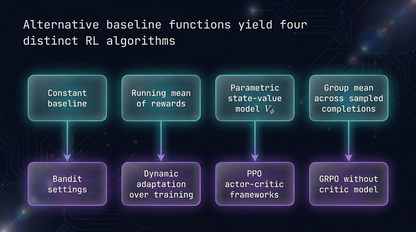
Fig 3. Baseline configurations establish distinct reinforcement learning algorithm families.
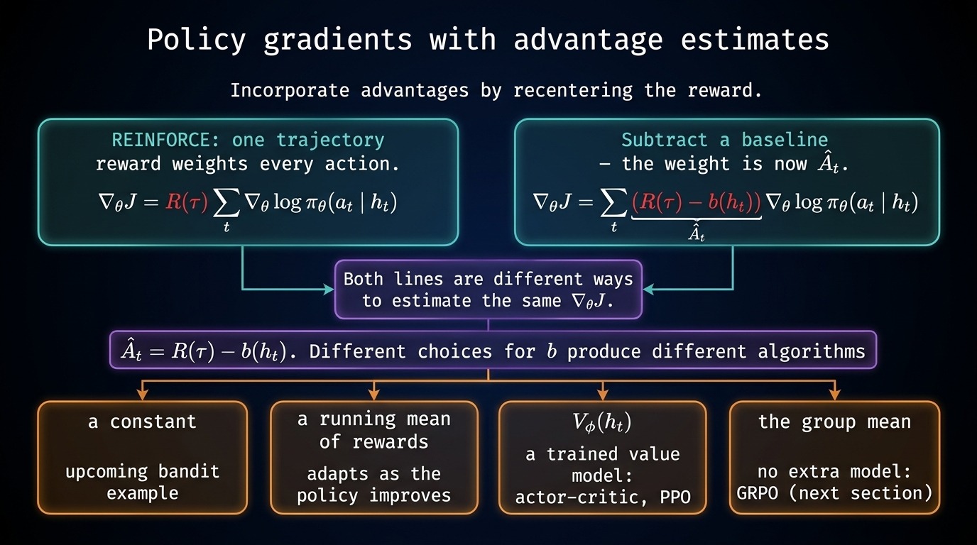
Fig 4. Centering trajectory rewards around baselines yields practical policy gradient advantage estimators.
Subtracting baselines recenters rewards to reduce sample variance without altering expected gradients. This stabilizes policy updates.
2.3 Proof of Zero Gradient Bias
History-conditioned baselines introduce zero estimation bias while significantly reducing variance across sampled trajectory updates.
- Express the expected value of the baseline-subtracted policy gradient estimator:
[\mathbb{E}\left[\widehat{\nabla_\theta J}\right] = \nabla_\theta J – \mathbb{E}\left[ \sum_t b(h_t) \nabla_\theta \log \pi_\theta(a_t \mid h_t) \right]] - Expand trajectory expectations using linearity into an outer expectation over histories and inner over actions:
[\mathbb{E}{a_t \sim \pi\theta}\left[ b(h_t) \nabla_\theta \log \pi_\theta(a_t \mid h_t) \right] = \sum_{a_t} \pi_\theta(a_t \mid h_t) b(h_t) \nabla_\theta \log \pi_\theta(a_t \mid h_t)] - Factor the action-independent baseline $b(h_t)$ outside the action summation:
[b(h_t) \sum_{a_t} \pi_\theta(a_t \mid h_t) \nabla_\theta \log \pi_\theta(a_t \mid h_t)] - Apply the log-derivative identity $\nabla_\theta \log \pi_\theta(a \mid h) = \frac{\nabla_\theta \pi_\theta(a \mid h)}{\pi_\theta(a \mid h)}$ to eliminate policy probabilities:
[b(h_t) \sum_{a_t} \nabla_\theta \pi_\theta(a_t \mid h_t)] - Interchange summation and gradient operators to take the gradient of total probability:
[b(h_t) \nabla_\theta \sum_{a_t} \pi_\theta(a_t \mid h_t) = b(h_t) \nabla_\theta (1)] - Differentiate constant 1 to zero, confirming the baseline term vanishes:
[\mathbb{E}\left[\widehat{\nabla_\theta J}\right] = \nabla_\theta J]
- History dependence requirement: Baselines must depend strictly on history $h_t$ rather than current action $a_t$.
- 1 total probability: Probabilities across the complete action space sum to exactly 1.
- 0 constant gradient: Gradients of constant values equal zero, eliminating the baseline term in expectation.
- Bias and variance: Baselines reduce empirical trajectory variance without introducing statistical bias into gradient calculations.
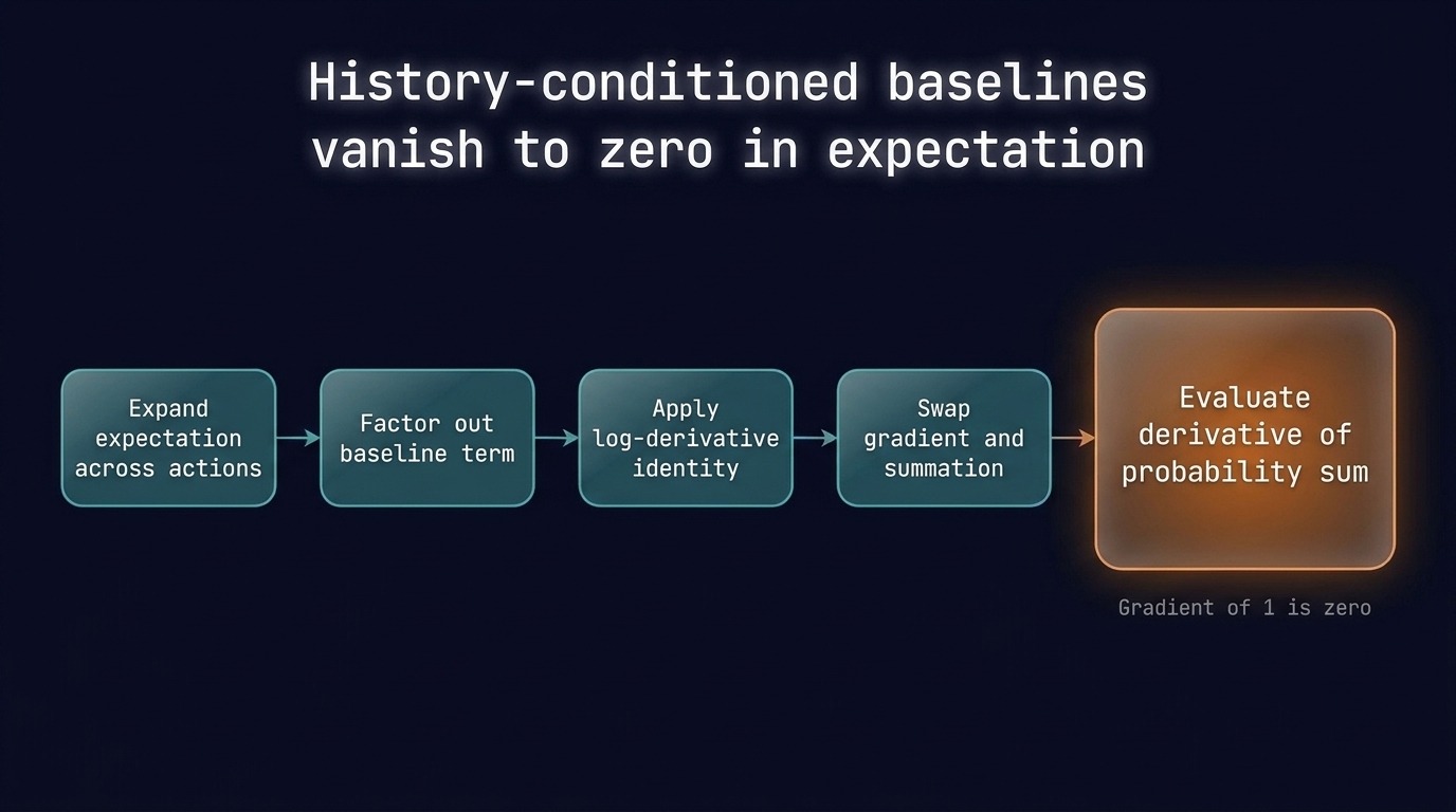
Fig 5. Action-independent baselines vanish in expectation because total action probability sums to one.
Baselines conditioned strictly on history avoid action correlations. This ensures policy gradients remain mathematically unbiased.
3. A Minimal Two-Armed Bandit Simulation
In short
– Baselines reduce gradient variance without shifting the expected policy gradient update.
– Centering rewards turns zero-reward failures into active corrective gradient signals.
– Scalar baselines cannot isolate credit among sequential actions in multi-step trajectories.
3.1 Bandit Parameterization and Setup
Daniel Fried examines baseline mechanics using a two-armed bandit (a simplified single-decision reinforcement learning setting).
- Single parameter $\theta$: scalar parameter controls action probabilities through a standard sigmoid squashing function.
- -1.1 initial value: starting parameter establishes a strong policy bias toward the failing action.
- 0.25 probability on A: guess A yields reward 1 but samples only one-quarter of runs.
- 0.75 probability on B: guess B yields reward 0 and dominates three-quarters of runs.
- Positive parameter shift: policy gradient (a method optimizing policy parameters via rewards) pushes $\theta$ upward.
[p = \pi_\theta(\text{guess } A) = \sigma(\theta) = \frac{1}{1 + e^{-\theta}}]
[1 – p = \pi_\theta(\text{guess } B) = 1 – \sigma(\theta) = 1 – p]
| Action | Probability | Reward | Log Derivative |
|---|---|---|---|
| Guess A | 0.25 | 1 | +0.75 |
| Guess B | 0.75 | 0 | -0.25 |
- Pass the current scalar parameter $\theta$ into the sigmoid activation function.
- Compute the resulting action probabilities $p$ and $1 – p$.
- Sample an action choice according to the computed probability distribution.
- Observe the numerical reward returned by the selected bandit arm.
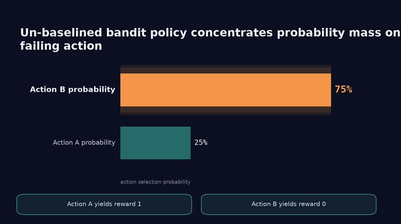
Fig 6. Action B dominates samples while Action A rarely yields reward.
Negative parameters squash sigmoid outputs below 0.5, concentrating probability on Action B. Shifting $\theta$ positive increases rewards.
3.2 Gradient Calculation Without Baseline
Calculating gradients without baselines produces noisy estimates that frequently stall policy parameter updates.
- +0.75 score derivative: derivative of log-probability evaluates to $1 – p$ for guess A.
- -0.25 score derivative: derivative of log-probability evaluates to $-p$ for guess B.
- +0.75 sampled update: sampling Action A scales positive derivative by full reward 1.
- 0.00 sampled update: sampling Action B zeroes out the gradient estimate entirely.
- 0.1875 analytical expectation: true expected gradient averages both sampled outcomes weighted by probability.
- 75% stalled rate: three out of four samples generate zero parameter updates.
[\frac{\partial}{\partial \theta} \log \pi_\theta(\text{guess } A) = 1 – p = 1 – 0.25 = +0.75]
[\frac{\partial}{\partial \theta} \log \pi_\theta(\text{guess } B) = -p = -0.25]
[\hat{g}A = R \times \frac{\partial}{\partial \theta} \log \pi\theta(\text{guess } A) = 1 \times (+0.75) = +0.75]
[\hat{g}B = R \times \frac{\partial}{\partial \theta} \log \pi\theta(\text{guess } B) = 0 \times (-0.25) = 0]
[\mathbb{E}[\hat{g}] = p \cdot (+0.75) + (1 – p) \cdot (0) = 0.25 \times 0.75 + 0.75 \times 0 = 0.1875]
- Calculate log-probability derivatives with respect to the scalar parameter $\theta$.
- Multiply the sampled action derivative by the raw observed trajectory reward.
- Update parameter $\theta$ in proportion to the resulting stochastic gradient estimate.
Multiplying by zero reward zeroes out gradients, ignoring valuable failure data. This creates high variance across updates.
3.3 Centering Rewards With Baselines
Subtracting a baseline (a reference value subtracted from rewards) turns negative outcomes into active learning signals.
- 0.5 constant baseline: subtracting 0.5 centers binary rewards symmetrically around the reference anchor.
- +0.5 positive advantage: Action A generates positive advantage (a metric measuring relative outcome quality).
- -0.5 negative advantage: Action B generates negative advantage indicating worse than expected performance.
- +0.375 baselined gradient: Action A multiplies positive advantage by positive derivative, boosting $\theta$.
- +0.125 corrective gradient: Action B multiplies negative advantage by negative derivative, boosting $\theta$.
[\hat{A} = R – b]
[\hat{A}_A = 1 – 0.5 = +0.5]
[\hat{A}_B = 0 – 0.5 = -0.5]
[\hat{g}A = \hat{A}_A \times \frac{\partial}{\partial \theta} \log \pi\theta(\text{guess } A) = (+0.5) \times (+0.75) = +0.375]
[\hat{g}B = \hat{A}_B \times \frac{\partial}{\partial \theta} \log \pi\theta(\text{guess } B) = (-0.5) \times (-0.25) = +0.125]
[\mathbb{E}[\hat{g}] = 0.25 \times (+0.375) + 0.75 \times (+0.125) = 0.09375 + 0.09375 = 0.1875]
| Action | Reward | Gradient ($b=0$) | Gradient ($b=0.5$) |
|---|---|---|---|
| Guess A | 1 | +0.750 | +0.375 |
| Guess B | 0 | 0.000 | +0.125 |
| Expectation | – | 0.1875 | 0.1875 |
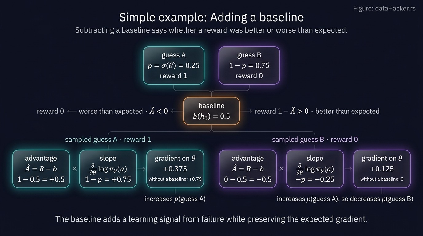
Fig 7. Centering rewards with a baseline triggers positive updates even from failures.
Two negative signs cancel when multiplying negative advantage by negative slope. Thus, failing actions actively push parameters correctly.
3.4 Variance Reduction and Convergence Paths
Baseline centering drastically reduces estimator variance while preserving identical mathematical expected gradient updates.
- 0.325 -> 0.108 standard deviation: subtracting constant baseline cuts gradient estimator dispersion by two-thirds.
- 0.1875 identical expectation: analytical mean remains precisely 0.1875 regardless of baseline choice.
- {0, 0.75} discrete spread: un-baselined estimator alternates between zero updates and large spikes.
- {0.125, 0.375} discrete spread: baselined updates remain close to the analytical expected gradient.
- 20-step empirical trial: un-baselined trajectories oscillate sharply compared to smooth baselined update trajectories.
- Initialize the policy parameter at scalar value $\theta = -1.1$.
- Draw twenty consecutive action samples from the parameterized distribution.
- Evaluate stochastic gradient updates with and without scalar baseline subtraction.
- Track cumulative parameter trajectories against the analytical expectation of 0.1875.
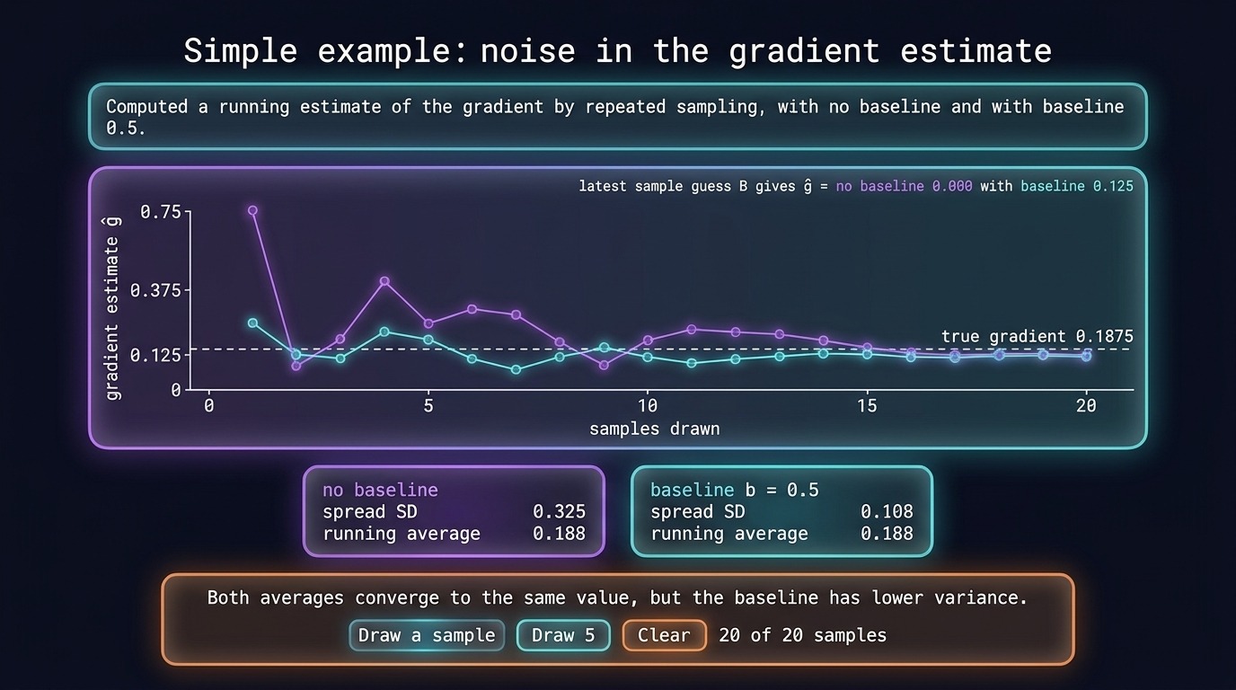
Fig 8. Baselined gradient trajectories exhibit substantially less noise across sample draws.
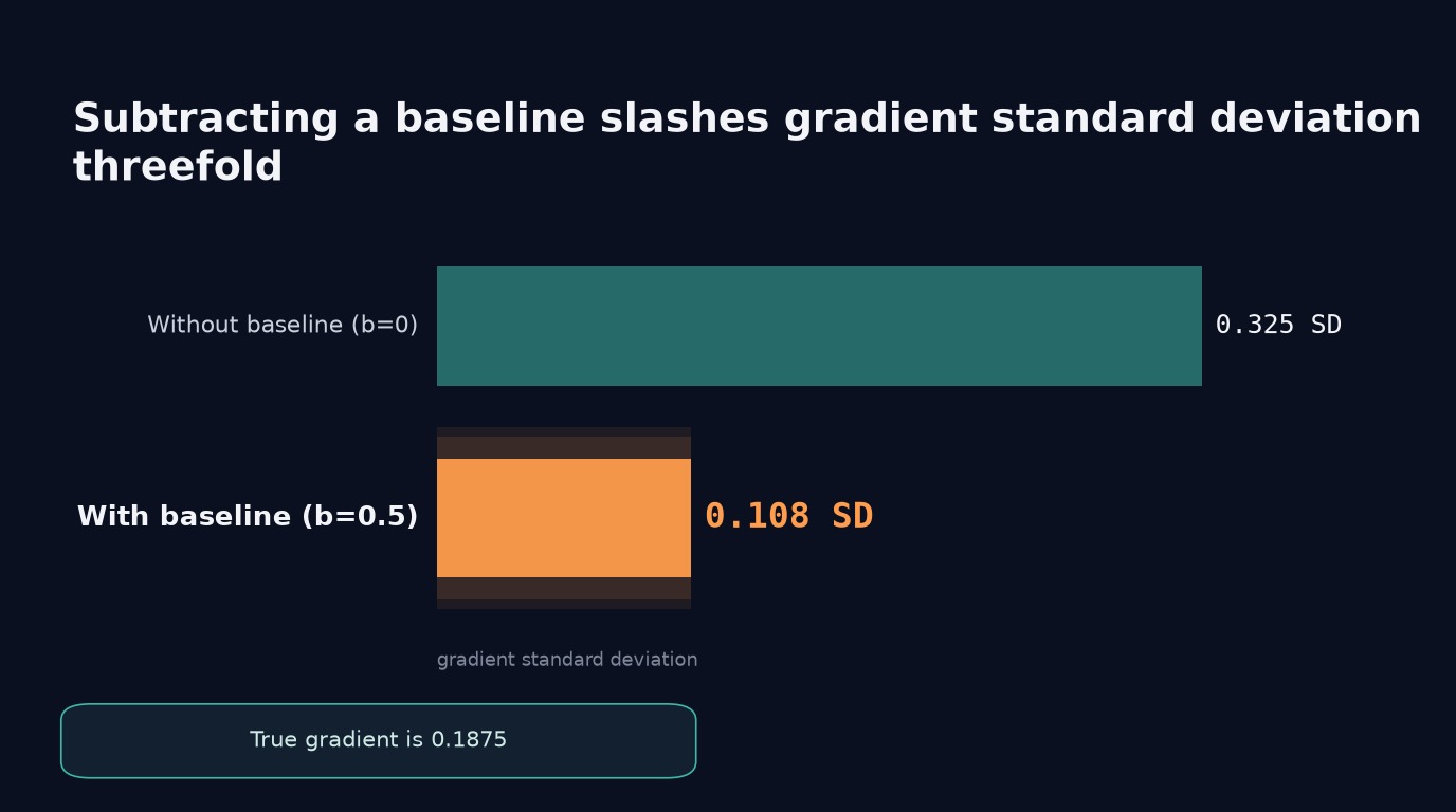
Fig 9. A constant baseline slashes standard deviation from 0.325 down to 0.108.
Subtracting a constant does not bias expectation because expected baseline derivatives integrate to zero. Reduced variance accelerates convergence.
3.5 Multi-Step Credit Assignment Limits
Scalar baselines benchmark overall trajectory performance but fail to resolve sequential action credit assignment.
- Uniform scalar advantage: every intermediate token receives the identical advantage value $\hat{A}$.
- Credit assignment limitations: scalar baselines cannot isolate which intermediate actions enabled success.
- 8, 12, 10, 11 guess chain: number guessing game shows identical credit applied across sequential attempts.
- +0.5 uniform credit: all four intermediate guesses receive identical reinforcement despite differing utility.
- Value model (Critic) requirement: state-dependent baselines $V^\pi(h)$ require training dedicated neural networks.
| Feature | Scalar Baseline | Critic Model |
|---|---|---|
| Computes Advantage | Trajectory-level | State-level |
| Resolves Credit | No | Yes |
| Training Cost | Zero | High |
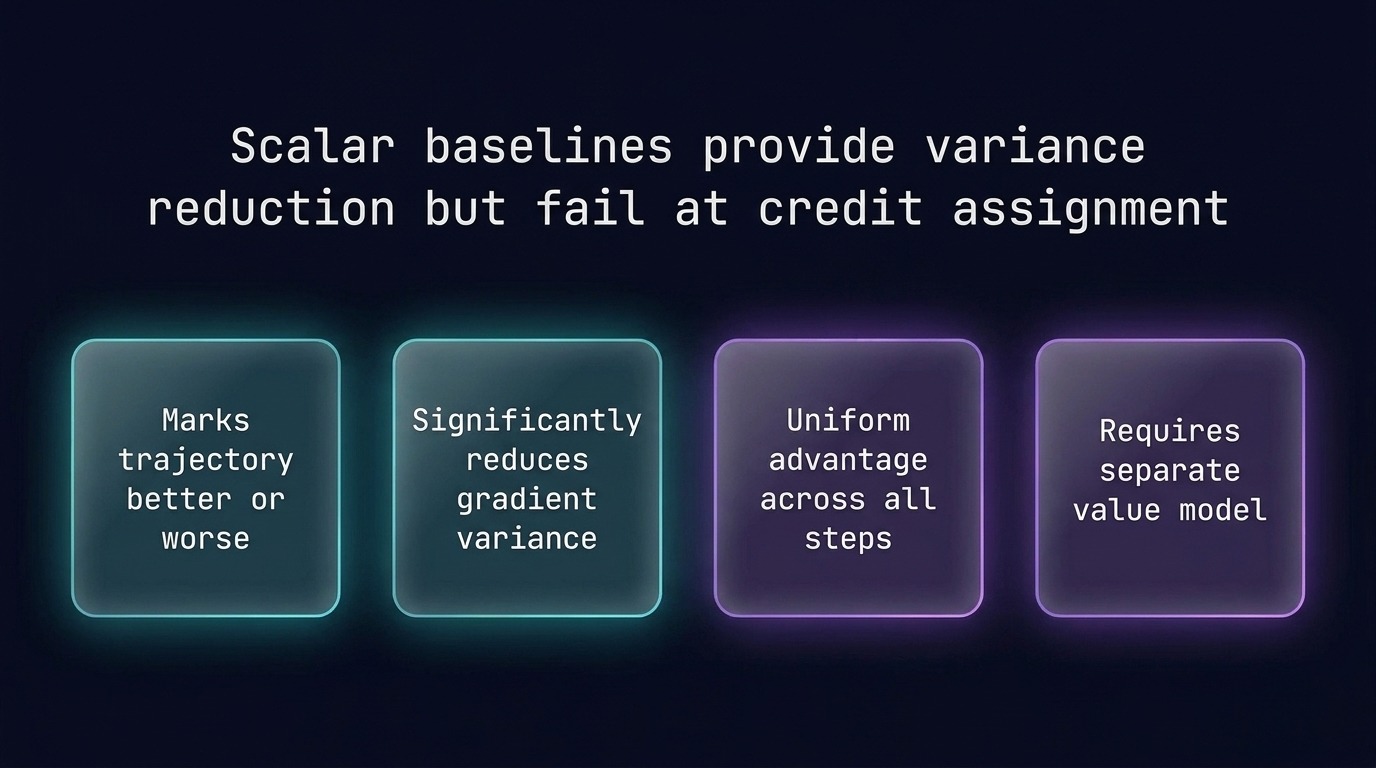
Fig 10. Scalar baselines stabilize updates but fail to resolve multi-step credit assignment.
Uniform rewards credit all intermediate actions equally regardless of their individual contribution. Sequential environments require state-dependent evaluation.
4. Intermediate Rewards: The Reward-to-Go Formulation
In short
– Reward-to-go weights each action using only subsequent rewards accumulated later in the trajectory.
– Dropping uninfluenced past feedback slashes gradient variance without introducing any update bias.
– Tasks with purely terminal payouts evaluate all intermediate steps using identical trajectory returns.
4.1 Filtering Future Returns with Reward-to-Go
Intermediate feedback environments benefit from reward-to-go (accumulating only subsequent rewards, filtering past payouts).
| Feature | Trajectory Return $R(\tau)$ | Reward-to-Go $R_t$ |
|---|---|---|
| Past tool reward (+0.2) | Included in update | Discarded from update |
| Terminal reward (+1) | Included in update | Included in update |
| Estimator variance | High gradient noise | Reduced update variance |
- $R_t$ formula: $R_t = \sum_{t’=t+1}^{T} r_{t’}$ sums rewards accumulated strictly after time step $t$.
- +0.2 tool reward: dropped from $a_t$ update because earlier feedback is unaffected by current choices.
- +1 terminal reward: retained in $R_t$ because downstream final payouts directly depend on action $a_t$.
- 8, 12, 10, 11 guesses: receive identical $R_t = R(\tau)$ returns when Number Search payouts occur terminally.
- Variance reduction: filtering out historical rewards produces cleaner policy gradient updates across multi-step sequences.
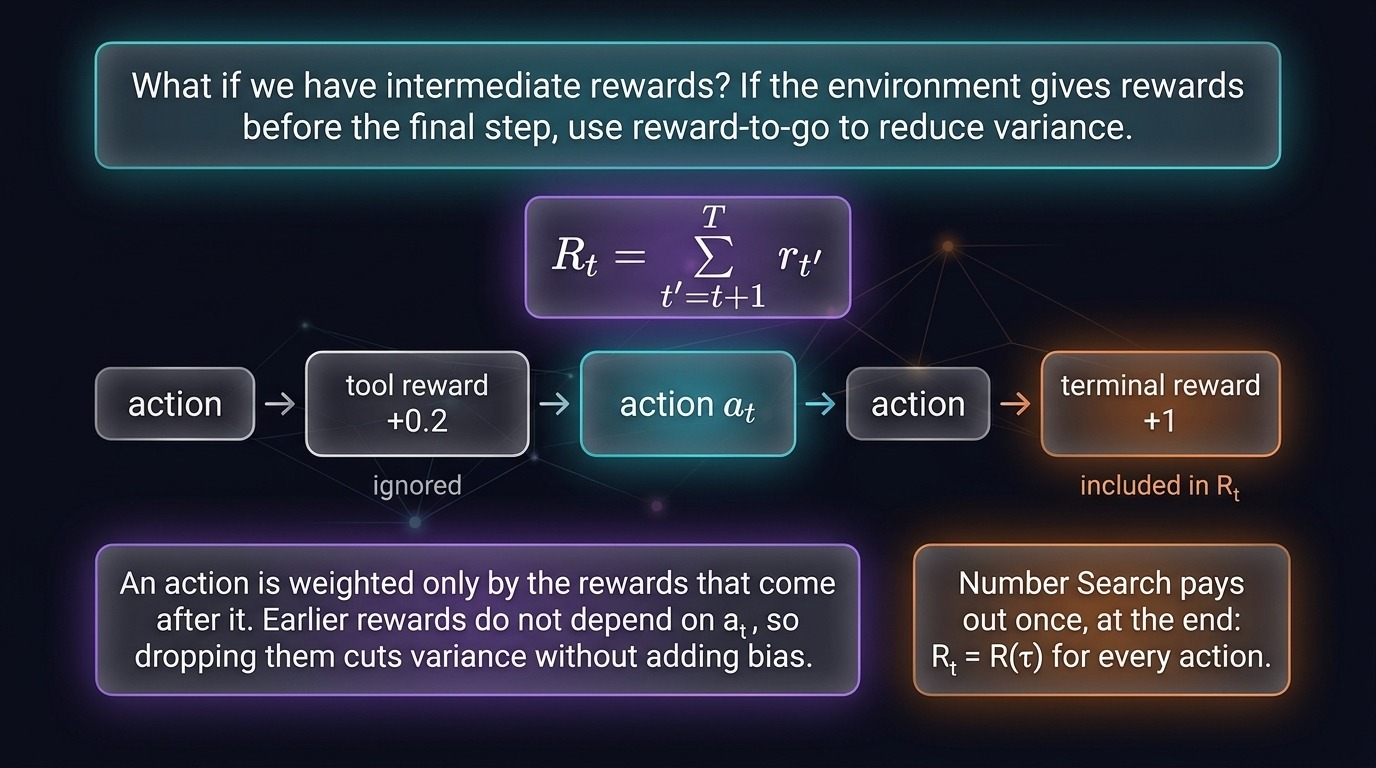
Fig 11. Reward-to-go lowers gradient variance by discarding past rewards from policy updates.
Past rewards cannot depend on the current action. Dropping them removes unnecessary noise without introducing estimator bias.
5. Group-Relative Policy Optimization (GRPO)
In short
– GRPO discards dedicated critic networks by sampling trajectory groups directly per prompt.
– Trajectory advantages normalize against empirical within-group return averages and standard deviations.
– Independent prompt grouping prevents difficulty distortions across heterogeneous training minibatches.
5.1 Eliminating Critics with Group Statistics
GRPO (Group-Relative Policy Optimization) [An algorithm that computes advantages by comparing multiple rollouts generated from the same prompt, eliminating the need for a separate critic model.] samples rollout groups to form a baseline [A reference value subtracted from trajectory rewards to evaluate whether an outcome was better or worse than expected without biasing gradient updates.].
| Approach | Baseline Source | Advantage Scaling | Value Network Needed |
|---|---|---|---|
| PPO [An actor-critic reinforcement learning algorithm that relies on an auxiliary parametric value model to estimate baselines and advantages.] | Value model (Critic) [A dedicated neural network trained alongside a policy to predict expected future returns from a given state or history.] | Critic return error | Yes |
| GRPO | Empirical group mean | Group standard deviation | No |
| DrGRPO [A variant of GRPO that removes group standard deviation scaling and token-length division to prevent task difficulty distortion and length drift.] | Empirical group mean | Unscaled mean centering | No |
- 1 critic network eliminated: avoids training an auxiliary value network to compute baselines.
- Shao et al. DeepSeekMath: introduced GRPO to eliminate critic models during mathematical reasoning training.
- $G$ candidate rollouts: sampled directly from the policy model for each input prompt.
- Empirical group mean: serves as baseline return $\bar{R} = \frac{1}{G}\sum_{j=1}^G R(\tau_j)$ across rollouts.
Standard policy optimization requires baselines to reduce return variance across rollouts. Group empirical averages eliminate extra parameter overhead while preserving mathematically unbiased baseline expectations.
5.2 Calculating Trajectory Advantages in Practice
Empirical advantage [A metric measuring how much better a specific action or trajectory is compared to the policy’s average expected return.] estimates normalize trajectory returns within each sampled group.
- Sample $G$ complete candidate rollouts from the policy for the input prompt.
- Score each trajectory outcome to obtain empirical scalar reward $R(\tau_j)$.
- Calculate empirical baseline mean $\bar{R} = \frac{1}{G} \sum_{j=1}^G R(\tau_j)$.
- Compute standard deviation $\sigma_R = \operatorname{std}{R(\tau_1), \dots, R(\tau_G)}$.
- Center rewards and divide by standard deviation: $\hat{A}_j = \frac{R(\tau_j) – \bar{R}}{\sigma_R}$.
- Number guessing game: an agent discovers a hidden target number through sequential guesses.
- 4 sampled trajectories: rollouts $\tau_1$ and $\tau_2$ succeed while $\tau_3$ and $\tau_4$ timeout.
- $R = 1$ for $\tau_1$ and $\tau_2$: guesses 8, 12, 10, 11 receive positive success rewards.
- $R = 0$ for $\tau_3$ and $\tau_4$: guesses 16, 8, 9, 10 or 1, 2, 3, 4 fail.
- $\bar{R} = 0.5$ and $\sigma_R = 0.5$: centered rewards equal $+0.5$ for successes and $-0.5$ for failures.
- $\hat{A} = +1$ versus $-1$: successes receive positive advantage while failures receive negative updates.
- Degenerate group [A rollout sample where all trajectories achieve identical rewards (all successes or all failures), resulting in zero advantage and stalled gradient updates.]: yields zero variance and produces no gradient update.
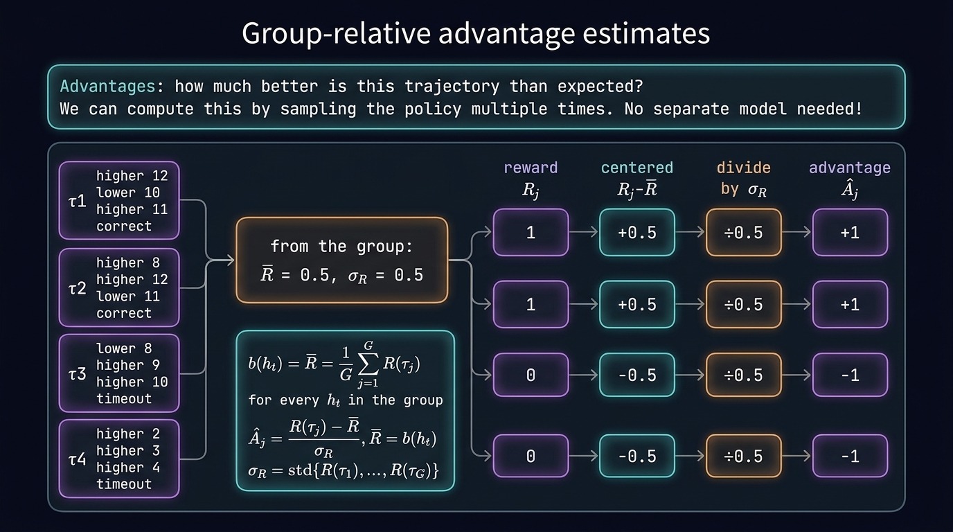
Fig 12. Group rollouts compute empirical return statistics to evaluate relative trajectory advantage without critics.
Group baselines remain mathematically unbiased because baselines depend strictly on prompts rather than individual actions. DrGRPO omits standard deviation scaling to prevent distorting optimization gradients across varying prompt difficulties.
5.3 Batching Multi-Prompt Rollouts
Minibatches contain multiple distinct task instances, each generating an isolated group of repeated rollout trajectories.
- 8 rollouts per group: practical setting noted by Fried for repeated prompt sampling.
- Isolated prompt statistics: each prompt $x_i$ evaluates independent mean $\bar{R}_i$ and standard deviation $\sigma_i$.
- 0.25 mean for hard tasks: prompt $x_2$ yields lower empirical return due to difficulty.
- 0.75 mean for easy tasks: simpler prompts achieve higher success rates across rollouts.
- Credit assignment [The challenge of determining which individual intermediate actions contributed to an overall outcome across a multi-step sequence.]: operates across multi-step sequential interactions within each task instance.
- Two-armed bandit [A simplified reinforcement learning environment where an agent makes a single discrete choice between two actions rather than a sequential chain of steps.]: contrasts with sequential guessing games by lacking multi-step states.
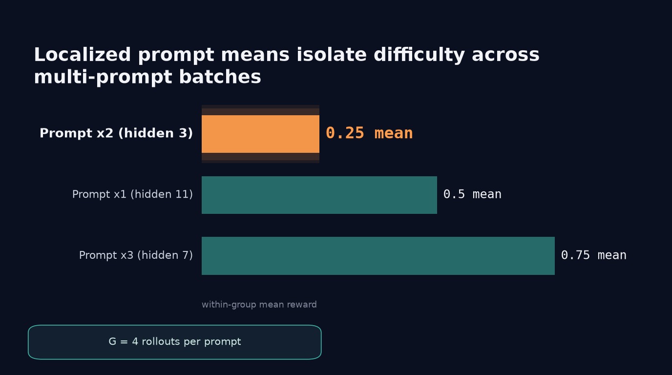
Fig 13. Isolating group statistics per prompt normalizes advantages across varied problem difficulty levels.
Computing baselines across full minibatches would unfairly penalize harder prompts with lower empirical rewards. Isolated group statistics ensure calibrated advantages tailored strictly to specific task complexity.
5.4 Policy Gradient Objectives and Updates
Policy gradient [A method that optimizes a policy’s parameters by adjusting action probabilities proportionally to observed rewards or advantages.] objectives rescale token log-probabilities using normalized group advantages.
Standard policy gradient loss:
[\mathcal{L}{\text{PG}}(\theta) = -\sum_i R(\tau_i) \sum_t \log \pi\theta(a_{i,t} \mid h_{i,t})]
GRPO policy gradient loss:
[\mathcal{L}{\text{GRPO}}(\theta) = -\sum_i \frac{1}{G} \sum{j=1}^G \hat{A}{ij} \sum_t \log \pi\theta(a_{ij,t} \mid h_{ij,t})]
- REINFORCE [A basic policy gradient algorithm that scales updates by the raw, unshifted trajectory reward, failing to actively penalize zero-reward failures.]: scales updates using unshifted raw returns rather than group advantages.
- Reward-to-go [A formulation where each action is weighted solely by rewards accumulated after that step occurs, filtering out irrelevant past rewards.]: weights individual tokens solely by subsequent rewards in trajectories.
- 1 advantage estimate $\hat{A}_{ij}$: rescales all action log-probabilities across rollout $j$ in prompt $i$.
- 3 omitted PPO mechanisms: excludes clipping mechanics, importance-sampling ratios, and KL-divergence penalties from DeepSeekMath.
- Empirical sample weights: adjust policy parameters directly from observed group performance.
Isolating empirical group advantages provides a practical mechanism to optimize policies without value networks. Reference model penalties and clipping prevent policy updates from taking excessively large gradient steps.
6. DrGRPO: Fixing Pathologies in Standard GRPO
In short
– DrGRPO removes standard deviation scaling to preserve true task difficulty awareness across groups.
– Constant budget division replaces response length normalization to prevent drift on wrong answers.
– Every token in a rollout shares the same unscaled, centered advantage coefficient.
6.1 Removing Standard Deviation and Length Normalization
DrGRPO modifies standard GRPO advantage scaling and token aggregation to eliminate two severe policy training biases.
| Component | Standard GRPO | DrGRPO |
|---|---|---|
| Advantage denominator | Group standard deviation $\sigma_R$ | None (raw centered $R_j – \bar{R}$) |
| Token normalizer | Variable response length $ | y_j |
| Instance weighting | Distorts easy and hard tasks | Preserves natural task difficulty |
| Length behavior | Drifts toward long wrong answers | Penalizes wrong answers equally |
- GRPO (Group-Relative Policy Optimization): an algorithm computing advantages by comparing multiple prompt rollouts without a separate critic.
- DrGRPO: a variant of GRPO removing group standard deviation scaling and token-length division.
- Advantage (relative outcome quality): a metric measuring how much better a specific action or trajectory is.
- Group standard deviation removal: unnormalized advantage $R_j – \bar{R}$ prevents easy or hard instances from inflating gradients.
- Response length division removal: replaces token count $\frac{1}{|y_j|} \sum_t (\cdot)$ with fixed maximum budget constant $\frac{1}{C} \sum_t (\cdot)$.
- Length drift prevention: fixed budget scaling stops policies from generating needlessly verbose incorrect answers.
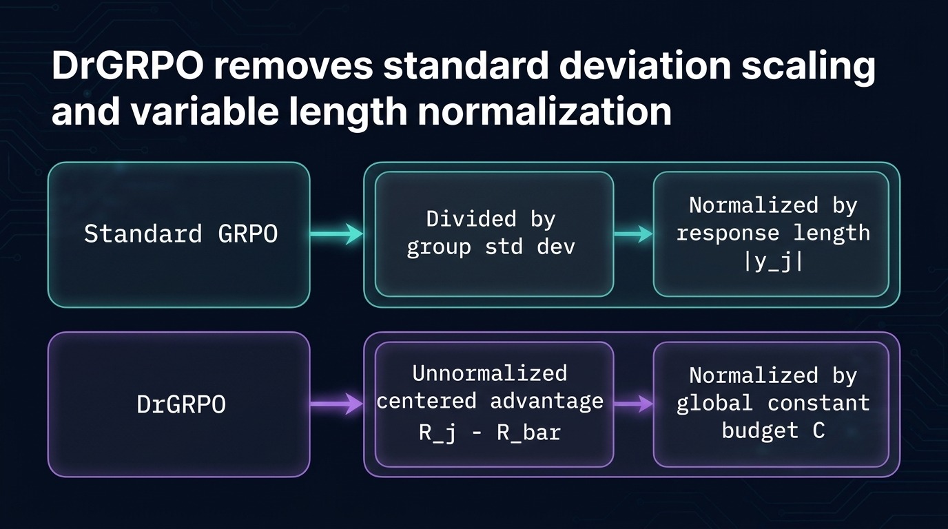
Fig 14. DrGRPO discards group standard deviation and variable length division to stabilize reinforcement training.
Small standard deviations on trivial or near-impossible prompts artificially inflate gradient updates. Variable length division inadvertently rewards verbosity on failing rollouts.
6.2 Per-Token Advantage Sharing Across Trajectories
Every token in a rollout receives an identical gradient weight based on its centered trajectory return.
- Unnormalized centered advantage: calculated directly for trajectory $\tau_j$ as $\hat{A}_j = R(\tau_j) – \bar{R}$ without standard deviation division.
- Uniform token weighting: assigns every generated token in rollout $\tau_j$ the identical coefficient $\frac{\hat{A}_j}{C}$.
- +0.5 / C token weight: assigned to actions
guess(8)andguess(11)when trajectory $\tau_1$ scores advantage $\hat{A}_1 = +0.5$. - -0.5 / C token weight: assigned to actions
guess(16)andguess(10)when trajectory $\tau_3$ scores advantage $\hat{A}_3 = -0.5$. - Aggregated DrGRPO loss: optimizes token probabilities across $G$ sampled rollouts where active tokens have mask $m_{j,t} = 1$:
[
\mathcal{L}{\text{DrGRPO}} = -\frac{1}{G} \sum{j=1}^G \frac{1}{C} \sum_{t: m_{j,t}=1} \hat{A}j \log \pi\theta(u_{j,t} \mid u_{j,<t})
]
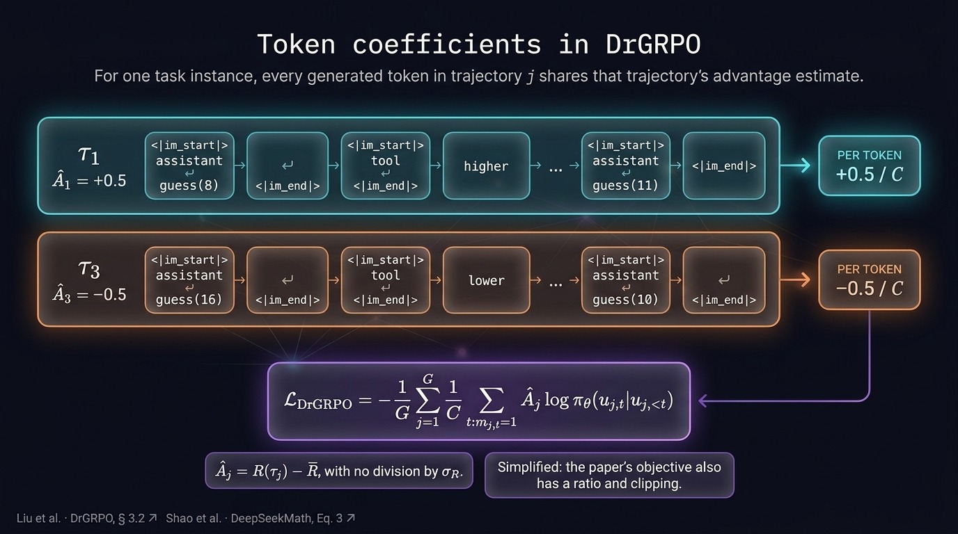
Fig 15. Every token in a trajectory shares a constant-divided centered advantage during policy updates.
Uniform token coefficients ensure credit spreads evenly across all sequential guesses in the game. This prevents later reasoning tokens from receiving disproportionate gradient penalties during optimization.
7. Failure Modes, PPO Comparison, and Unification
In short
– Degenerate groups yield identical rewards and zero gradients, requiring active intervention.
– GRPO discards critic networks by calculating baselines directly across sampled groups.
– Policy algorithms share an action-weighted gradient objective addressing exposure and data mismatch.
7.1 Degenerate groups and mitigations
Optimization stalls when rollouts in a sample return identical rewards without any empirical variance.
- [0, 0, 0, 0] rewards: all trajectories fail when tasks exceed the policy’s current capabilities.
- [1, 1, 1, 1] rewards: all trajectories succeed when tasks offer no challenge to the agent.
- 0 advantage: degenerate groups (rollouts with identical rewards) produce zero gradients under GRPO.
- Number guessing stall: guesses like 8, 12, and 10 all fail, yielding no comparative signal.
- Curriculum adaptation: adjusts task difficulty dynamically to restore reward spread across rollouts.
- Expert rollouts: injects demonstration trajectories directly into sample pools to guarantee non-zero success.
- Reward shaping: supplies intermediate feedback signals to score incremental multi-step guessing progress.
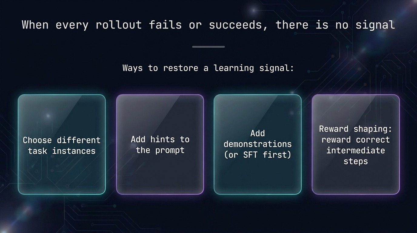
Fig 16. Interventions restore empirical variance when every sampled rollout in a group fails.
Zero advantage (a metric measuring how much better a trajectory performs versus average) halts updates entirely. Policy gradient (adjusting action probabilities proportionally to rewards) requires non-zero advantage variance to guide weight adjustments.
7.2 PPO versus GRPO architecture
GRPO replaces parametric value baselines with empirical advantage estimates computed across sampled output groups.
- Value model (Critic): dedicated neural network predicting expected future returns in PPO actor-critic setups.
- GAE computation: calculates advantage estimates using state baseline predictions from the auxiliary critic model.
- Shared backbones: standard PPO architectures couple policy and value heads, inflating memory overhead.
- G candidates: GRPO samples completions for prompt query $q$ without auxiliary value networks.
- Empirical baseline: baseline (a reference subtracted to evaluate relative performance) derives directly from completion returns.
- Memory savings: GRPO eliminates parameter synchronization costs between policy and dedicated critic networks.
| Feature | Standard PPO | GRPO |
|---|---|---|
| Critic model | Required separate value network | None; uses group statistics |
| Advantage calculation | Generalized Advantage Estimation | Group-relative score centering |
| Memory footprint | High (policy, value, reference) | Lower (policy and reference) |
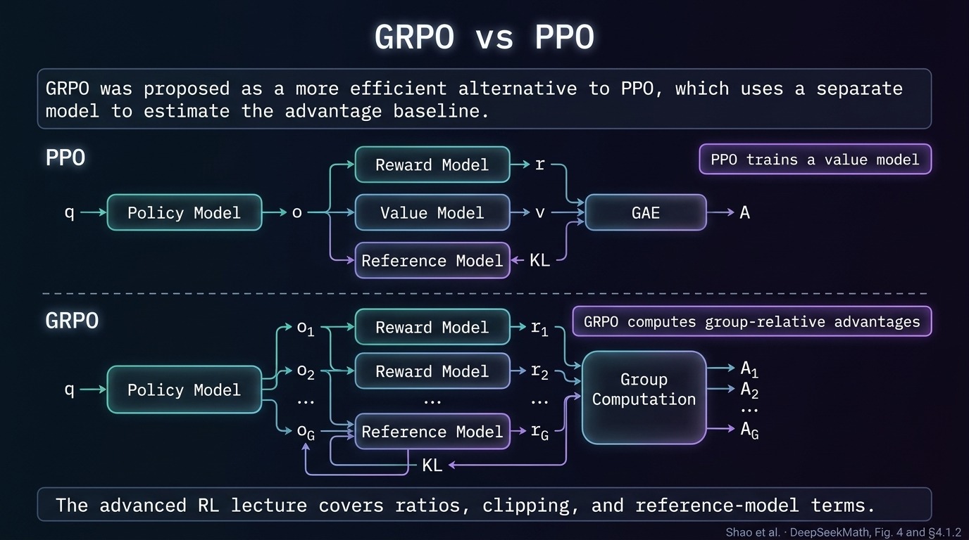
Fig 17. GRPO replaces critic networks with empirical group statistics computed across candidate trajectories.
Separate critic networks require massive compute and encounter severe training instabilities during fine-tuning. Group estimation circumvents parametric baseline fitting by measuring performance relative to peer rollouts.
7.3 Unified policy action weighting
Policy gradient formulations and self-training methods unify under a shared action-weighted optimization objective.
[\widehat{\nabla_\theta J} = \sum_t w_t \, \nabla_\theta \log \pi_\theta(a_t \mid h_t)]
- REINFORCE weighting: scales steps by raw episode return without actively penalizing complete failures.
- ReST-EM weighting: filters trajectories with binary indicators, executing supervised updates strictly on successes.
- GRPO weighting: weights actions by group-relative advantages normalized across multiple completions.
- DrGRPO weighting: removes standard deviation divisors to prevent distorted task difficulty scaling.
- Two-armed bandit: simplified reinforcement learning decisions illustrate how relative weighting shifts action selections.
- Reward-to-go: credit assignment (attributing multi-step outcomes to specific choices) isolates rewards after each step.
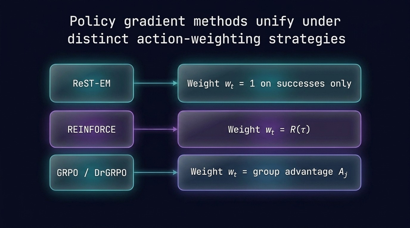
Fig 18. Policy gradient and self-training objectives differ strictly through their chosen action weights.
The unified objective reweights token log-probabilities using trajectory outcomes to guide parameter updates. The specific choice of weight $w_t$ governs credit assignment and update magnitude across tokens.
| Algorithm | Action weight ($w_t$) | Baseline mechanism |
|---|---|---|
| REINFORCE | Raw trajectory return $R$ | None |
| ReST-EM | Binary success indicator $\mathbb{I}_{\text{success}}$ | Filter threshold |
| PPO | Critic-based GAE $\hat{A}_t$ | Parametric value model |
| GRPO | Group-normalized return $\tilde{A}_i$ | Empirical group mean |
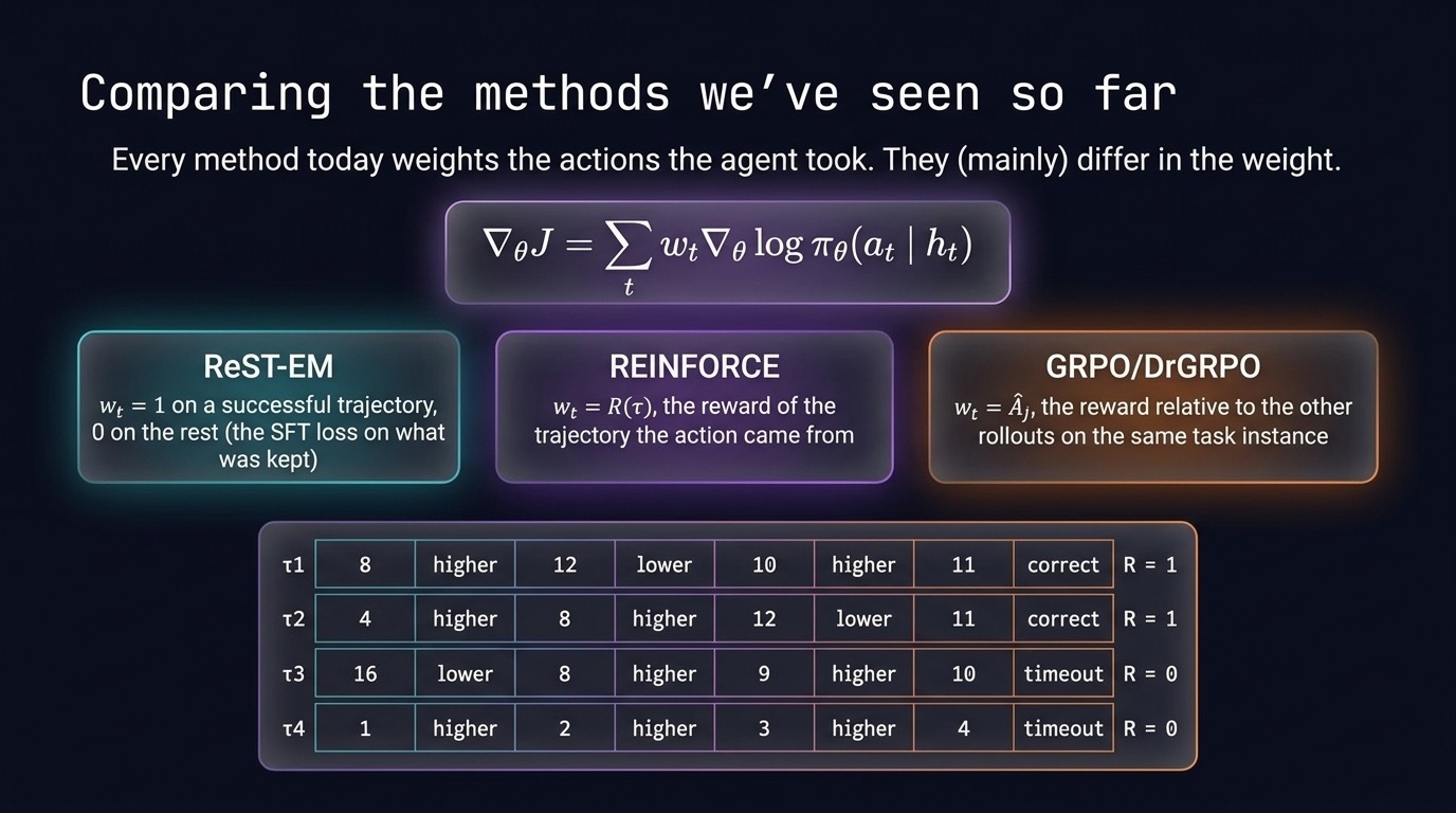
Fig 19. Reinforcement methods systematically vary their advantage baselines and sample filtering mechanisms.
Different reinforcement learning objectives select distinct weighting functions to optimize policy updates. The selected weighting mechanism dictates computational complexity and gradient variance during training.
7.4 Core reinforcement learning benefits
Sampling trajectories directly from active policies and weighting by relative reward resolves structural training bottlenecks.
- Task mismatch: directly optimizes expected reward so any successful sequence receives positive reinforcement.
- Data mismatch: relative baselines extract constructive gradient signals even from sub-optimal rollout batches.
- Exposure bias: on-policy sampling forces models to encounter mistakes and learn recovery steps.
- Target discovery: number guessing policies learn error corrections when guesses overshoot target values.
On-policy exploration prevents distribution drift by evaluating states the current policy actually generates. Reweighting trajectories ensures agents systematically favor high-reward actions across sequential decisions.
8. Summary
- Degenerate groups: identical group rewards yield zero advantage, requiring curriculum, demonstrations, or shaped rewards.
- GRPO efficiency: empirical group-relative statistics eliminate memory overhead and training instability of value models.
- Unified gradients: foundational algorithms share a policy gradient template varying solely in action weights.
- Distribution alignment: on-policy trajectory sampling resolves task mismatch, data mismatch, and autoregressive exposure bias.
Source
Lecture: Reinforcement Learning Basics by Daniel Fried, Carnegie Mellon University.
Course: CMU 11-768 AI Agents (Fall 2026), Lecture 9, second half. The first half is covered in LLM_log #038.
Video: YouTube · Slides: PDF · Course page: cmu-agents.com
Further reading referenced in the lecture:
dataHacker.rs — LLM_log #039: Policy Gradient Baselines — From REINFORCE to GRPO. By Vladimir Matic.