LLMs from Scratch #003: Modern Transformer Architectures: A Deep Dive into Design Principles and Training
Modern Transformer Architectures: A Deep Dive into Design Principles and Training
🎯 What You’ll Learn
In this comprehensive guide, we’ll explore the evolution of transformer architectures from the original “Attention is All You Need” paper to modern implementations. You’ll discover why today’s language models use specific design choices like RoPE position embeddings and SwiGLU activations, understand the trade-offs between serial and parallel layer arrangements, and learn how to make informed decisions about hyperparameters like head dimensions and aspect ratios. By examining the collective wisdom from hundreds of trained models, you’ll gain practical insights into what makes transformers work at scale.
Tutorial Overview
- Course Overview and Architecture Philosophy
- Contemporary Model Landscape
- Layer Organization and Block Architecture
- Position Embedding Approaches
- Attention Head Configuration
1. Course Overview and Architecture Philosophy
Understanding modern transformer architectures requires more than just learning the original paper. The field has evolved dramatically since “Attention is All You Need” was published, with hundreds of models providing empirical evidence about what actually works at scale. This journey begins with understanding how we got from the vanilla transformer to today’s state-of-the-art implementations.
Course Goals and Starting Point
Welcome to this deep dive into transformer architectures and training. This lecture has been titled “everything you didn’t want to know about LLM architecture and training” because we’re going to get into some of the nitty-gritty details that most other classes would spare you from—questions like what should my hyperparameters be? What architectural choices actually matter?
We’ll start with a quick recap of the transformer architecture, giving you two variants: the standard transformer you might see in CS224N, and then the modern consensus variant that you actually implement in practice. From there, we’ll take a much more data-driven perspective to understanding transformer architectures.
The central question: People have trained lots of LLMs at this point, and you can read all those papers to understand what has changed and what has remained common. Through this almost evolutionary analysis, we can try to understand what are the things that are really important to make transformers work. Today’s theme follows the class philosophy that the best way to learn is hands-on experience, but since we can’t train all these transformers ourselves, we’ll learn from the experience of others.
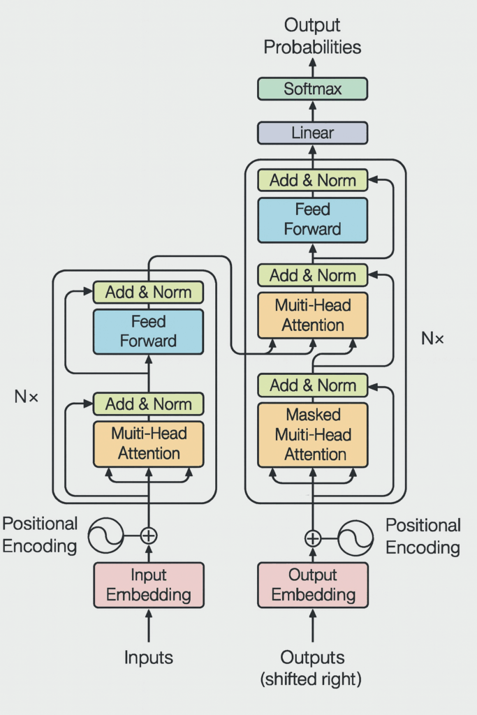
Our starting point is the original transformer with its simple position embeddings at the bottom, multi-head attention, layer norms afterwards, a residual stream going upwards, an MLP, and softmax at the very end. We’re going to see variants to all these different pieces until we get to the most modern transformer variants.
💡 Key Architectural Formulas
The original positional encoding uses sine and cosine functions at different frequencies to capture both higher and lower frequency positional information:
$$PE_{(pos,2i)} = \sin(pos/10000^{2i/d_{\text{model}}})$$
$$PE_{(pos,2i+1)} = \cos(pos/10000^{2i/d_{\text{model}}})$$
The feed-forward network in the original transformer applies a simple two-layer transformation with ReLU activation:
$$\text{FFN}(x) = \max(0, xW_1 + b_1)W_2 + b_2$$

This can be seen as a vanilla transformer block. Yet, over the years numerous tiny changes have been applied.
🔴 Learning From Collective Experience
The philosophy driving this course is simple: The best way to learn is through hands-on experience. Since we can’t train all these transformers ourselves, we learn from the experience of others. By examining hundreds of published language models, we can perform an almost evolutionary analysis to understand which components are truly essential for transformer success.

One example of the modern transformer block
Modern Design Principles Emerge
The landscape of large language models has exploded in recent years. We’ve seen the emergence of Command R, small language model variants, and the Gemma series. When you start looking deeper into what’s available, the sheer volume becomes overwhelming—from Gemma 3 and Qwen 2.5 to countless other architectures.
The Challenge of Model Proliferation
The proliferation of language models has reached a point where keeping track of them all has become a significant challenge in itself. This explosion represents both an exciting opportunity and a practical challenge for researchers and practitioners. Each model brings different strengths, architectures, and use cases to the table.
However, from this diversity, we can extract common design principles that have proven successful across different implementations. This data-driven approach to understanding transformers forms the foundation of modern architecture design.
2. Contemporary Model Landscape
Now let’s dive into the current state of dense language models, where we’ve seen an explosion of innovation with about 19 new model releases in the last year alone. Many of these releases include minor architecture tweaks, but collectively they represent a wealth of information since not all models pursue the same approaches. This rapid development is evident when examining the technical reports and publications from major AI research organizations, showcasing the intense pace of architectural experimentation across the field.
Dense Architecture Variations and Data
The landscape has become remarkably diverse. When you start looking deeper into what’s available, the sheer volume becomes overwhelming—you’ll find Gemma 3 and Qwen 2.5, and honestly, you can’t even cover the screen with all these different models. The proliferation of language models has reached a point where keeping track of them all has become a significant challenge in itself.
This explosion of models represents both an exciting opportunity and a practical challenge for researchers and practitioners. There’s simply a lot of models out there now, each with different strengths, architectures, and use cases. The field has moved from having a handful of notable language models to an ecosystem so rich and varied that comprehensive coverage requires significant effort and resources.
Convergent Evolution in Neural Architectures
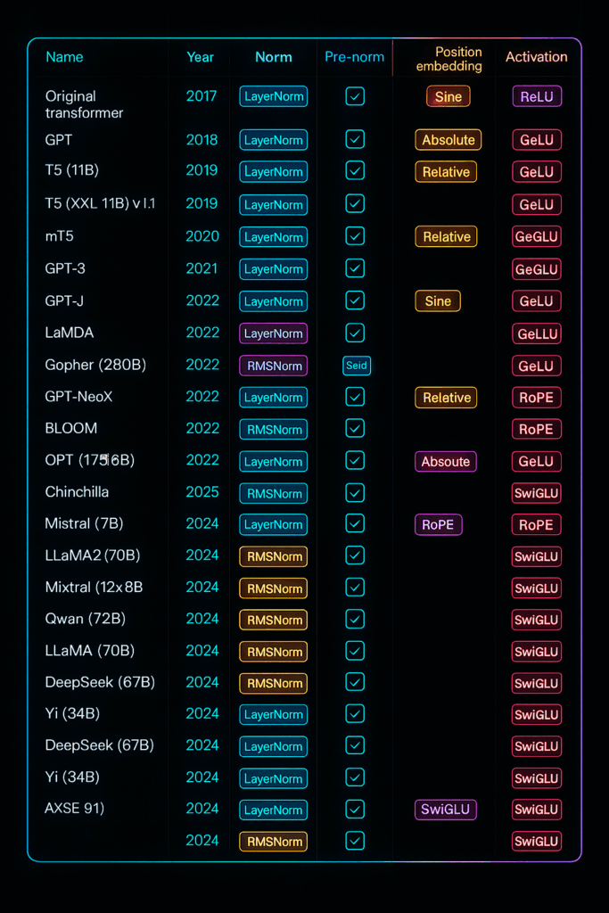
To make sense of this architectural diversity, a comprehensive spreadsheet tracking what all these models are doing becomes essential—spanning from the original transformer in 2017 all the way to the newest models in 2025. What emerges is a fascinating pattern of convergent evolution in neural architectures.
Take position embeddings as an example: researchers used to experiment with all sorts of approaches including absolute, relative, RoPE, and even ALiBi for some teams. However, starting around 2023, virtually everyone has converged on RoPE as the standard approach. This convergence tells us something important about what actually works at scale.
Three Major Sections of Design Decisions
This lecture will cover three major sections focusing on the key decisions in modern language model design, each critical to understanding how to build effective transformers at scale.
💡 Architecture, Hyperparameters, and Training
First: Architecture Variations – We’ll explore activations, feed forwards, attention variants, and position embeddings. These are the fundamental building blocks that determine how information flows through your model and how effectively it can learn from data.
Second: Intelligent Hyperparameter Selection – Once we’ve nailed down the architecture, we need to intelligently select hyperparameters. Questions arise like: How big to make the hidden dimension? What size to use for the \(ff\_dim\) in the MLP projection layer? Whether \(multi\_head\) dimensions should always sum to \(model\_dim\)? How many vocabulary elements to include? These aren’t choices you want to pick out of a hat—they have significant implications for model performance and computational efficiency.
Third: Training Strategy – The approach to training, including optimization techniques, learning rate schedules, and other critical decisions that affect whether your model converges to a good solution.
🔴 The State of Architectural Consensus
Two important observations emerge from this analysis:
First, there’s still not much consensus on many architectural choices, despite some convergent evolution toward what we might call “LLaMA-like architectures” in recent years. Researchers continue to experiment with different approaches—swapping between LayerNorm and RMSNorm, choosing between serial versus parallel layer arrangements, and exploring various activation functions.
While there’s one choice that basically everyone has adopted since the very first GPT (which we’ll explore in detail), the landscape remains rich with variations that we can learn from. Each variation offers insights into the optimal design space for large language models, and by studying these patterns, we can make more informed decisions about our own architectures.
The remainder of this guide will systematically walk through these choices, examining the evidence for each decision and understanding not just what works, but why it works.
3. Normalization Strategies
One of the most fundamental architectural decisions in modern transformers involves how and where we apply normalization. This seemingly simple choice has profound implications for training stability, convergence speed, and final model performance. Let’s explore the evolution of normalization strategies and understand why the field has converged on certain approaches.
Pre-Norm vs Post-Norm: A Critical Architecture Choice
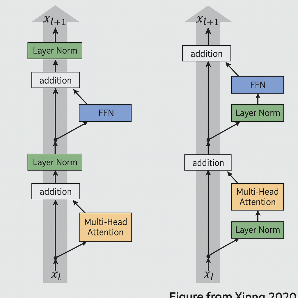
The original transformer paper used a post-norm approach where you had your residual stream, and layer norms were applied after every subcomponent. They would do multi-head attention, add back to the residual stream, then layer norm that result. The same pattern applied to the fully connected layer.
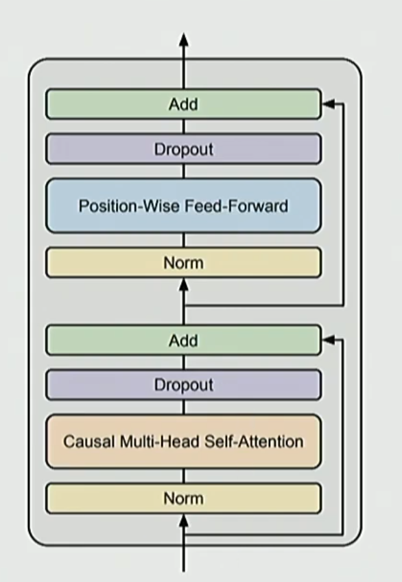
Very early on though, people realized that moving the layer norm to the front of the non-residual part performed much better in many different ways. Basically, almost all modern transformer models use this pre-norm approach (right image below).
Training Stability: Why Pre-Norm Won
The motivation for this pre-versus post-norm shift comes down to training stability. If you wanted to use post-norm, it was much less stable and required careful learning rate warm-up to train properly. Early papers by Salazar and Yen, along with Xiong’s 2020 work, consistently showed that pre-norm with other stability tricks could eliminate the need for warm-up while achieving equal or better performance than post-norm with careful warm-up approaches.
💡 Gradient Behavior Insights
The arguments centered around gradient behavior across layers. With pre-norm, gradient sizes remained constant, whereas post-norm without warm-up would cause gradients to blow up.
Early work by Salazar and Yen identified that post-norm training showed many more loss spikes and generally unstable behavior. You’d see gradient norms spiking and remaining higher throughout training compared to the smoother pre-norm approach. This reinforced the view of pre-norm and other layer norm tricks as essential stability-inducing aids for training neural networks.
In the image below, note that we have used the double norm layers (see below), that became the standard in many architectures in 2024.
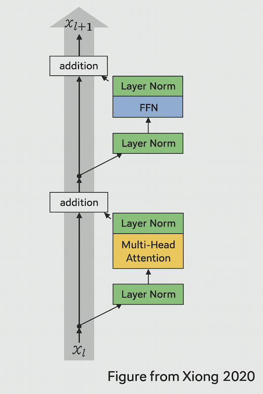
🔴 The Double Norm Innovation
Recently, there’s been a new innovation called “double norm”—a variant that didn’t exist when this material was first presented. While we know putting layer norms directly in the residual stream is bad, recent models like Grok and Gemma II have started adding layer norms both before and after the transformer blocks.
Some models like Llama II only add layer norm after the feed-forward and multi-head attention components. This approach has shown some promise for improved stability in larger models, though pre-norm had been dominant for quite a while.
LayerNorm vs RMSNorm: The Efficiency Revolution
Now let’s examine another critical normalization decision that has reshaped modern transformer architectures. Many models used LayerNorm and it worked quite well
Norm equation
$$y = \frac{x – \mathbb{E}[x]}{\sqrt{\text{Var}[x] + \epsilon}} * \gamma + \beta$$
RMS norm equation
$$y = \frac{x}{\sqrt{||x||_2^2 + \epsilon}} * \gamma$$
and there’s been a consensus change—basically all modern models have switched to RMSNorm.
What is RMSNorm?
RMSNorm simplifies the normalization process by dropping the mean adjustment. You don’t subtract the mean and you don’t add a bias term $\beta$. Notable models like the Llama family, PaLM, Chinchilla, and T5 have all moved to RMSNorm.
Why the switch? One reason is that it doesn’t really make a difference—if you train models with RMSNorm, it performs just as well as LayerNorm, so there’s a simplification argument.
The Real Argument: Speed and Memory
The real argument often given in papers is that RMSNorm is faster and just as good. If you don’t subtract the mean, that’s fewer operations. If you don’t have to add that bias term $\beta$ back, that’s fewer parameters to load from memory into your compute units.
Now, you might be thinking—didn’t you tell us that only matrix multiplies matter for runtime? And this isn’t a matrix multiply, so why should we care?
If you look at the percentage of flops taken up by different operations in a transformer, tensor contractions (matrix multiplies) are about 99.8% of the flops. So saving 0.17% of flops doesn’t seem like a huge win.
🔴 Memory Movement: The Hidden Bottleneck
Here’s the key insight for architecture design: You can’t just think about flops—you also have to think carefully about memory movement.
Even though tensor contractions are 99.8% of the flops, operations like softmax and layer norms represent only 0.17% of flops but actually take up 25% of the runtime! The big reason is that these normalization operations incur a lot of memory movement overhead.
So it does matter to optimize these lower-level operations, because it’s not just about flops—it’s about memory movement. When we talk about GPU architectures, thinking about memory becomes very, very important, not just flops.
This table shows the comparison of different Norms and final loss results. 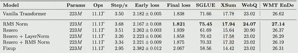
💡 Concrete Performance Gains
This is one reason why RMSNorm has become much more popular. Narang et al. in 2020 had a nice ablation study showing concrete results:
- Vanilla transformer: 3.5 steps per second
- With RMSNorm: 3.68 steps per second
Not a huge gain, but it’s essentially free. And you get a final loss that’s actually lower than the standard transformer. So we’ve gotten runtime improvements and, in this case, even loss improvements—that’s a win-win situation for us.
Bias Terms and Implementation Simplicity
Building on this trend toward simpler, more efficient architectures, let’s examine another important implementation detail that follows the same principles as RMSNorm. Most modern transformers do not have bias terms.
The Original FFN with Bias Terms
The original transformer feed-forward network would have your inputs $X$ going through a linear layer with a bias term, then ReLU it, and then a second linear layer wrapping around it:
$$\text{FFN}(x) = \max(0, xW_1 + b_1)W_2 + b_2$$
But most implementations, if they’re not gated units, actually just drop the bias terms entirely. You can make this argument from basically the same kinds of underlying principles—they perform just as well, and matrix multiplies are apparently all that you need to get these models to work.
The other thing, which is maybe more subtle, is actually optimization stability. There have been really clear empirical observations that dropping these bias terms often stabilizes the training of these largest neural networks. So now a lot of implementations omit bias terms entirely and train only on these pure matrix multiply settings.
Generalizable Lessons in Architecture Design
This trend extends beyond just bias terms. Basically everyone does pre-norm or at least they do the layer norms outside of the residual stream, which gives you nicer gradient propagation and much more stable training.
Most people, or almost everybody, does RMS norm in practice because it works almost as well as layer norm but has fewer parameters to move around. This idea of dropping bias terms just broadly applies—a lot of these models just don’t have bias terms in most places.
While deep learning has been very empirical and bottom-up rather than top-down, there are some generalizable lessons we can draw from these details. The lesson of having very direct identity map residual connections is a story that has played out in many different kinds of architectures, and the effectiveness of layer norm has been consistently demonstrated. Not letting your activations drift in scale is another thing that has been very effective for training stability.
These patterns represent fairly generalizable lessons that extend beyond transformers. We also see systems concerns come into play again, which is another generalizable lesson about thinking really carefully about the impact of your architecture on the systems components of your design. The trend toward simpler, more stable architectures without bias terms, combined with techniques like RMS normalization, reflects a broader understanding of what makes large neural networks trainable and efficient.
4. Activation Functions and Gating Mechanisms
Moving from normalization to activation functions, we enter another critical design space where architectural choices significantly impact model performance. The landscape of activation functions is surprisingly diverse, and understanding which ones work best—and why—is essential for building effective transformers.
The Activation Function Zoo
There’s a whole big zoo of activations: ReLU, GELU, Swish, GLU, and many others. And then there are different kinds of MLPs: GeGLU, ReGLU, SwiGLU, and more variants.
The bottom line? It really does matter—SwiGLU and other GLU variants consistently work well, and you should think about them carefully because they do work and you should internalize that pattern.
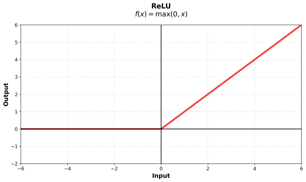
Standard Activation Functions
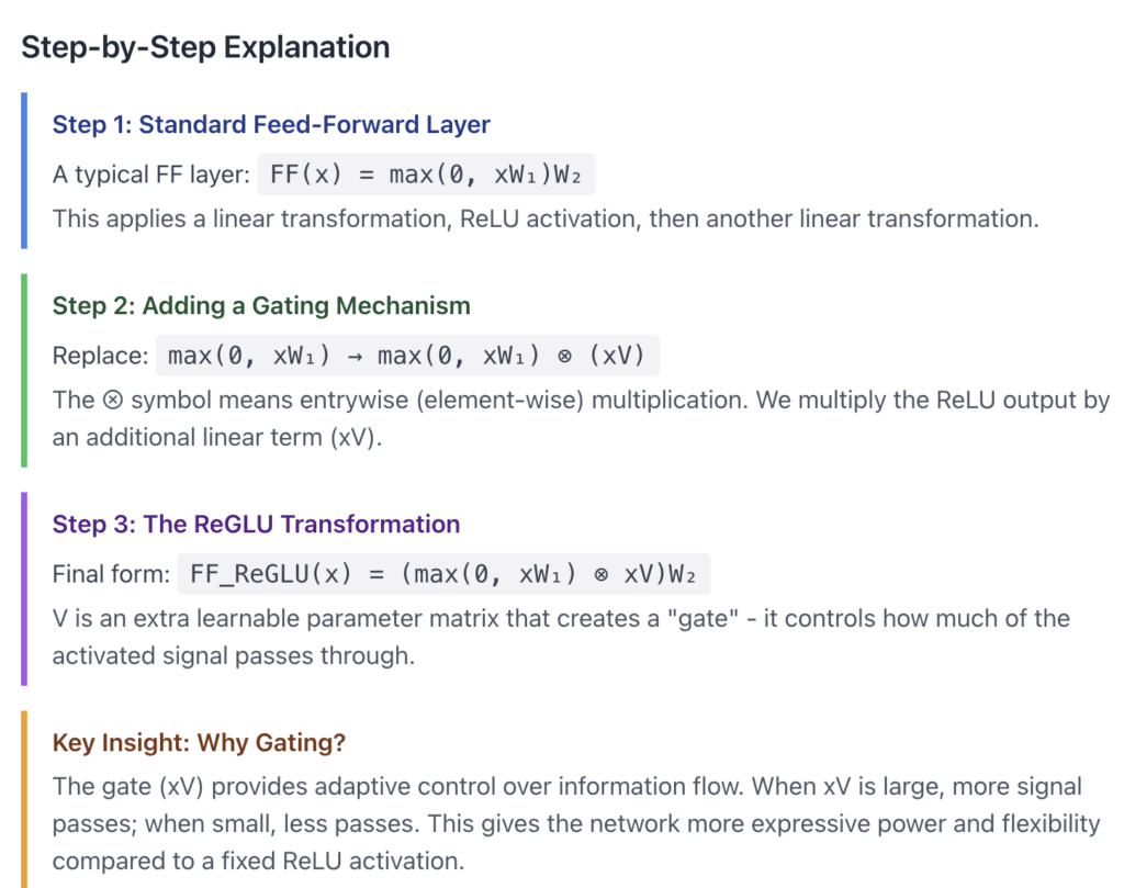
Let’s start with the basics. ReLU is the activation you learn in the most basic deep learning classes. You just take the max of 0. In the case of the MLP (dropping bias terms), you’ve got \(x \cdot W_1\), you take the ReLU, and then you do \(W_2\):
$$\text{FF}(x) = \max(0, xW_1) W_2$$
GELU (Gaussian Error Linear Unit) is a more sophisticated alternative. This one multiplies the linear function with the CDF of a Gaussian. So it’s basically going to be like ReLU, but with a little bit of a bump at the bottom. This makes things a little bit more differentiable, which may or may not help:
$$\text{FF}(x) = \text{GELU}(xW_1)W_2$$
$$\text{GELU}(x) := x\Phi(x)$$
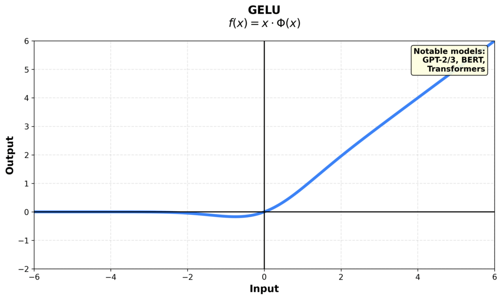
💡 Historical Adoption Patterns
The GPT family of models (GPT-1, GPT-2, GPT-3, and GPT-J) all use GELU. The original transformer and some of the older models used ReLU, but really almost all the modern models have switched to the gated linear units, like SwiGLU and GeGLU.
The Google folks really pushed for this approach with PaLM and T5, and since it’s been tried and true, basically almost all models post-2023 use a gated linear unit.
Gated Linear Units (GLU): The Modern Standard
So what makes gated linear units special? This is another place where gating appears and proves to be a very good way of doing things. Gating has emerged as one of those consistently useful architectural patterns, alongside residual connections and layer norms.
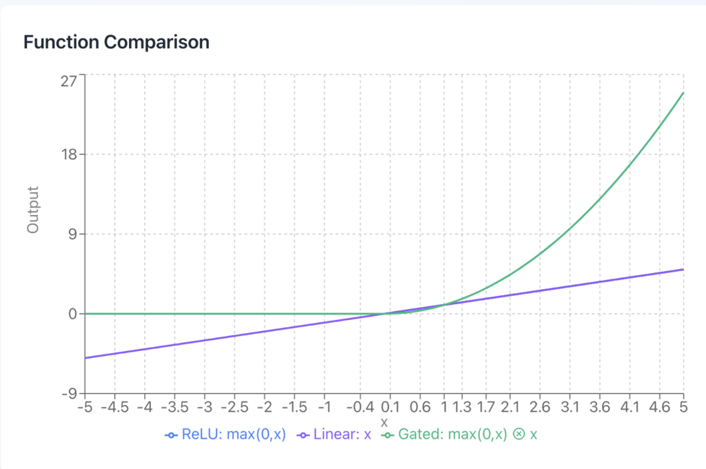
From Standard FF to Gated Variants
Originally, we had our fully connected layer with ReLU. GLUs modify the “first part” of a feedforward layer. Now, instead of doing just linear and ReLU, what we do is gate the output with an element-wise linear term:
$$y_i^{(x)} = \max(0, xW_1) \cdot xW_2$$
This introduces gating where you’re multiplying the ReLU activation by another linear transformation. The element-wise product ($\otimes$) creates a gating mechanism that allows the model to control information flow more flexibly.
💡 SwiGLU and GeGLU Variants
Different GLU variants use different activation functions in the gating mechanism:
$$\text{GeGLU}(x) = (\text{GELU}(xW) \otimes xV)W_2$$
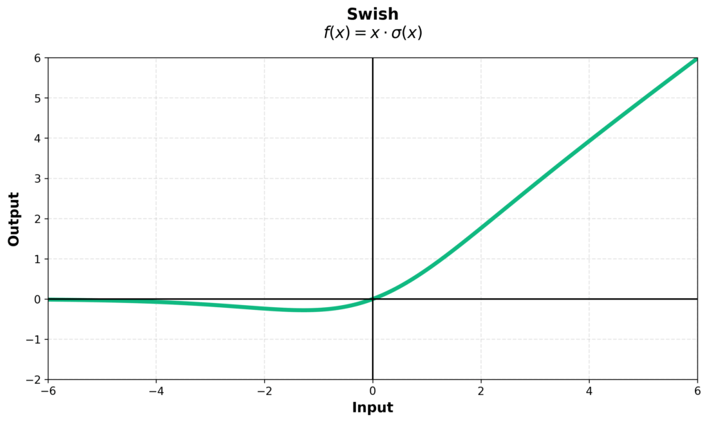
$$\text{SwiGLU}(x) = (\text{Swish}_1(xW) \otimes xV)W_2$$
where Swish is defined as \(x \mapsto x \cdot \text{sigmoid}(\beta x)\).
Addressing Concerns About Non-Monotonic Activations
A natural question arises about these activation functions: since both the swish function and the gating function aren’t monotonically increasing—in fact, they’re decreasing in certain regions—wouldn’t this cause problems with gradient descent?
🔴 Why Non-Monotonicity Isn’t a Problem
There’s a small negative region to the left of zero where the derivative flips direction, which intuitively might seem problematic and could potentially trap activations at zero.
However, in practice, neural network optimization dynamics involve high learning rates with momentum, so you’re not really going to converge to that zero point. The activations end up being distributed all over the place, so this tiny negative piece doesn’t have a huge practical effect on the model.
Parameter Sizing for GLU Variants
One important consideration when implementing gated linear units is parameter sizing. Since we’ve added this extra \(V\) parameter matrix, we need to think carefully about how to size these components.
💡 The Two-Thirds Rule
The standard practice is to make the hidden size—basically the output dimensionality of \(W\)—slightly smaller by a factor of two-thirds compared to non-gated counterparts.
This ensures that the total number of parameters in the entire gated system remains the same as the non-gated versions. It’s a conventional approach that most practitioners follow: for gated linear units, you simply make everything a bit smaller to maintain parameter matching across different architectures.
GLU Performance in Practice
Before diving into the performance results, let’s address a practical question about computational overhead. One of the benefits of GELU functions is their easy differentiability with respect to input. If you have the derivative of the CDF for a Gaussian distribution, which involves terms like \(e^{-x^2}\), does that significantly slow things down?
Computational Overhead Analysis
What really matters here is the memory pressure, and it will be exactly the same when you’re reading the same level of elements. So the extra computational overhead is negligible anyway, and actually the memory calculus remains the same.
It’s entirely possible that SwiGLU or GELU might be implemented with lookup tables internally in CUDA. The bottom line is that these concerns don’t manifest as practical bottlenecks.
Empirical Evidence: GLU Variants Win
Gated linear units clearly work. Looking at Shazeer’s original paper evaluating all these GLU variants, the evidence is compelling. Looking at CoLA and SST-2 performance, the GLU variants consistently perform better, with scores of 84.2, 84.12, 84.36, and 84.67.
They even provide standard deviations so you can determine how significant those results are, and they are indeed statistically significant.
There was also the Narang et al. 2020 paper, which is an excellent study of various architecture variants in the context of T5-style models. Once again, you see that the gated linear unit variants consistently achieve lower losses than their counterparts—notice that the bolded lines correspond exactly to the GLU variants. This pattern has basically held up across different studies, making gated linear units widespread and dominant in modern architectures.
In short, there are many papers that demonstrated that GLU has become almost a default activation function to use.
🔴 GLU Isn’t Strictly Necessary, But…
Of course, GLU isn’t strictly necessary for a good model—just because it’s probably slightly better and everyone uses it doesn’t mean it’s essential. You can find examples of very high-performance models that don’t use GLU:
- GPT-3: No GLU, still high performance
- Nemotron 340B: Uses squared ReLU
- Falcon 2 11B: Uses standard ReLU
These are all relatively high-performance models, showing that GLU isn’t absolutely required. However, the evidence does point toward somewhat consistent gains from SwiGLU and GeGLU variants, which is why modern implementations use exactly those variants.
There are many variations across models—ReLU, GELU, and various GLU implementations—but the gated approaches have proven their worth through consistent performance improvements across the field. This convergence toward gated activations, alongside the adoption of pre-norm and RMSNorm, represents another example of the field learning from collective experience what actually works at scale.
5. Layer Organization and Block Architecture
Now let’s explore one of the most significant architectural variations in modern transformers—how we arrange and connect the layers themselves. This seemingly simple choice has profound implications for both model performance and computational efficiency at scale.
Serial Layer Arrangements: The Traditional Approach
Traditionally, transformer blocks operate in a serial fashion. For each block, outputs come in from the bottom, you perform your attention computation, pass that result forward, then do your MLP, and pass that computation forward. This inherently serial approach means you do attention first, then MLP—one after the other in sequence.
However, this serial connection can create certain parallelism constraints when you want to distribute computation across gigantic sets of GPUs, potentially leading to lower GPU utilization and more difficult systems concerns. These limitations have motivated researchers to explore alternative arrangements.
The traditional serial formulation can be written mathematically as:
$$y = x + \text{MLP}(\text{LayerNorm}(x + \text{Attention}(\text{LayerNorm}(x))))$$
Parallel Layers: A Systems-Driven Innovation
To address the limitations of serial processing, several models have adopted what we call parallel layers. Instead of having serial computation of attention and MLP, they perform both operations simultaneously. You take your input \(x\) from the previous layer, compute both the MLP and attention side by side, then add them together into the residual stream for your output.
This approach was pioneered by GPT-J, an open source replication effort, and the folks at Google were bold enough to implement this at really large scale with PaLM, with many others following since.
The parallel formulation changes the computation flow to:
$$y = x + \text{MLP}(\text{LayerNorm}(x)) + \text{Attention}(\text{LayerNorm}(x))$$
💡 Computational Advantages of Parallel Architectures
When implemented correctly, this parallel formulation offers significant advantages. You can share LayerNorm computations, fuse matrix multiplications together, and achieve systems efficiencies that result in roughly 15% faster training speed at large scales.
The MLP and attention input matrix multiplications can be fused, leading to better GPU utilization. Ablation experiments showed small quality degradation at 8B scale but no quality degradation at 62B scale, suggesting the effect should be quality neutral at even larger scales like 540B parameters.
🔴 Current Adoption Status
Despite these advantages, parallel layers haven’t been quite as popular in recent years. Most models we’ve seen in the last year have used serial layers rather than parallel ones. The main exceptions include Cohere’s Command-R and Command-R Plus, along with Falcon 2 11B.
This trend suggests that while parallel layers offer clear computational benefits, the transformer community has largely settled on the traditional serial approach for most applications. The reasons for this preference relate to both implementation complexity and the trade-offs between computational efficiency and model expressiveness.
💡 Serial vs Parallel Efficiency
When asked whether serial is more efficient than parallel, it’s actually the reverse—parallel is more efficient than serial, which is why people are willing to make this architectural choice despite potential expressiveness trade-offs.
In some sense, you might expect serial processing to be more expressive because you’re composing two computations rather than adding them together. However, the benefit of parallel architectures lies in computational efficiency through kernel fusion and shared computations.
When you write the right kinds of fused kernels, many of these operations can be executed in parallel, and computation can be shared across different parallel components. This parallel formulation results in roughly 15% faster training speed at large scales since the MLP and Attention input matrix multiplications can be fused.
Ablation experiments showed a small quality degradation at 8B scale but no quality degradation at 62B scale, suggesting the effect should be quality neutral at the 540B scale. These implementation details help us understand the broader patterns we see across the entire landscape of modern architectures.
Architecture Design Summary
When we examine the evolution of neural network architectures over the past several years, fascinating patterns emerge in how researchers have approached fundamental design decisions. The landscape has been dominated by transformer-based models, but the specific architectural choices have varied significantly across different implementations and research groups.
What’s particularly interesting is how certain design patterns have become more prevalent over time. We see a clear trend toward pre-normalization techniques, which help with training stability, and the adoption of more sophisticated position embedding methods. The activation functions have also evolved, with many modern architectures moving beyond simple ReLU to more advanced alternatives like GELU and SwiGLU.
6. Position Embedding Approaches
One of the most fundamental questions in transformer design is: how do we encode positional information? Unlike recurrent networks that process sequences sequentially, transformers operate on all tokens in parallel. This parallelism enables much faster training but creates a challenge—the model has no inherent notion of token order. Position embeddings solve this problem, and the evolution of these techniques tells a fascinating story about architectural innovation.
Absolute Position Embeddings: The Original Approach
The earliest models like GPT-1, GPT-2, GPT-3, and OPT used absolute embeddings, which simply add a learned position vector to the token embedding:
$$\text{Embed}(x, i) = v_x + u_i$$
This straightforward approach directly encodes positional information but lacks the ability to generalize well to sequences longer than those seen during training. If your model trains on sequences of length 512, it has no learned representation for position 513 and beyond.
The original “Attention is All You Need” paper introduced an elegant alternative using sinusoidal functions:
$$\text{Embed}(x, i) = v_x + PE_{pos}$$
where the positional encoding is defined as:
$$PE_{(pos,2i)} = \sin(pos/10000^{2i/d_{\text{model}}})$$
$$PE_{(pos,2i+1)} = \cos(pos/10000^{2i/d_{\text{model}}})$$
💡 Why Sine and Cosine?
The sinusoidal position encodings use different frequency ranges to capture both higher and lower frequency positional information. Lower frequency components (with larger wavelengths) can represent coarse positional information over long distances, while higher frequency components capture fine-grained local position distinctions.
This mathematical formulation allows the model to potentially extrapolate to sequence lengths longer than those seen during training, since the sine and cosine functions are defined for all positions.
Relative Position Embeddings: T5 and Gopher
Some models like T5 and Gopher took a different path, implementing various kinds of relative embeddings that add vectors directly to the attention computation. These relative position embeddings modify the attention mechanism itself:
$$c_{ij} = \frac{x_i W^Q (x_j W^K + a_{ij}^T)^T}{\sqrt{d_z}}$$
where \(a_{ij}\) represents the relative position information between tokens \(i\) and \(j\). This approach allows the model to focus on relative distances between tokens rather than their absolute positions in the sequence.
7. Rotary Position Embeddings (RoPE)
Let’s dive into one of the most elegant solutions to position encoding in modern transformers: Rotary Position Embeddings, or RoPE. This approach represents a fundamental rethinking of how we encode positional information, and its widespread adoption tells us something important about its effectiveness.
The Core Intuition: Relative Positions Matter
The high-level thought process behind RoPE is that what matters is the relative positions of vectors. If I have an embedding \(f(x, i)\), where \(x\) is the word I’m trying to embed and \(i\) is my position, then I should be able to write things down in this way:
There should exist a function \(f\) such that if I take the inner product of \(f(x, i)\) and \(f(y, j)\), I can write this down as some different function \(g(x, y, i-j)\), which depends on the two words and the difference in their positions:
$$\langle f(x, i), f(y, j) \rangle = g(x, y, i-j)$$
This definition enforces absolute position invariance—you only pay attention to how far apart these two words are.
When you check existing approaches like sinusoidal embeddings, you get cross terms that are not relative, so you still leak absolute position information:
$$\langle \text{Embed}(x, i), \text{Embed}(y, j) \rangle = \langle v_x, v_y \rangle + \langle PE_i, v_y \rangle + …$$
Relative embeddings are relative but not inner products, violating our constraint. RoPE is this clever observation that we know one thing that is invariant to absolute things: rotations. We’re going to exploit that structure to come up with our position embeddings, leveraging the fact that inner products are invariant to arbitrary rotation.
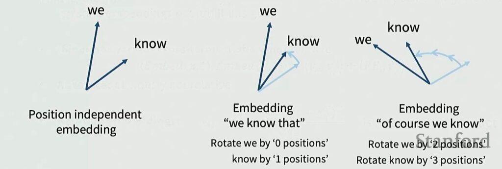
💡 A Concrete Example: “We Know”
Let me illustrate with an example. Say my embedding for the word “we” is this arrow, and my embedding for “know” is this other arrow.
For the sequence “we know that”:
- “we” is at position 0 → I don’t rotate it at all
- “know” is at position 1 → I rotate it by one unit of rotation
For the sequence “of course we know”:
- “we” and “know” have the same relative positioning but are shifted by two positions
- “we” → I rotate by 2 positions
- “know” → I rotate by 3 positions
If you look at these two arrow pairs, they have the same relative angle, so their inner products are preserved!
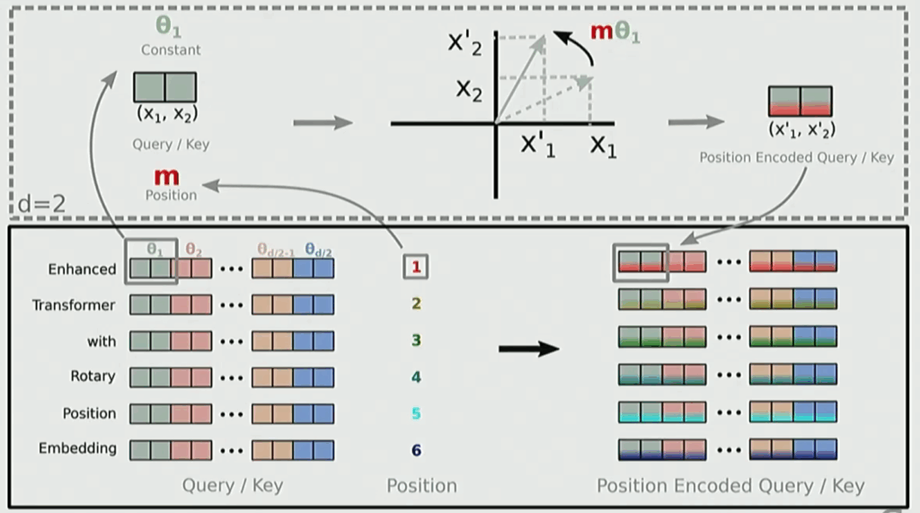
From 2D Intuition to High-Dimensional Implementation
This is the nice idea about RoPE—you just rotate the vectors, with rotation angle determined by each word’s position. Since inner products don’t care about relative rotations, these inner products only look at the difference in distance.
🔴 The High-Dimensional Challenge
While it’s easy to think about in 2D where there’s only one way to rotate a vector, in high-dimensional spaces where we operate, it’s not obvious how to do this rotation.
The RoPE approach came up with the simplest but effective way: take your high-dimensional vector of dimension \(d\) and cut it into blocks of 2 dimensions. Every 2-dimensional pair gets rotated by some \(\theta\), creating a rotation speed for each pair.
Much like sinusoidal embeddings, you pick different \(\theta\) values so some embeddings rotate quickly while others rotate slowly, capturing both high-frequency close-by information and low-frequency distant positioning information. The actual RoPE math involves multiplying with sinusoidal rotation matrices—rotations are just matrix multiplies, so they don’t create computational issues.
RoPE Mathematical Foundation
Now that we understand the intuition behind RoPE, let’s dive into the mathematical machinery that makes it work. The core mathematical operation in RoPE involves multiplying your embedding vectors with two-by-two block matrices, creating a purely relative positioning system.
The Rotation Matrix Structure
Since the \(\theta\) values are fixed and the matrices \(M\) are predetermined, this essentially becomes a fixed matrix multiplication with your vector. The beauty of this approach lies in its simplicity—there are no additive or cross terms that complicate the computation.
When considering which trigonometric functions to use, the key insight is to pair up coordinates and rotate them in 2D space, drawing motivation from complex number representations.
The rotation matrix for RoPE is applied to the query and key projections:
$$f_{\{q,k\}}(x_m, m) = R^d_{\Theta,m} W_{\{q,k\}} x_m$$
where $R^d_{\Theta,m}$ is the rotation matrix containing cosine and sine terms with various angle parameters $m\theta_1, m\theta_2, \ldots, m\theta_{d/2}$.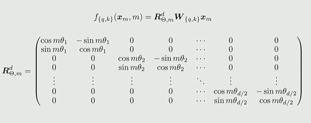
💡 Implementation Simplicity
From an implementation perspective, this approach avoids computational complexity because you’re not learning the $\theta$ parameters themselves. If you were optimizing these angles, you’d face the challenge of differentiating through trigonometric functions, but RoPE sidesteps this issue entirely by keeping them fixed.
The $\theta$ values that determine the rotation angles are hyperparameters, not trained parameters. Much like in the sines and cosines, there’s a schedule to the rotation angles that are determined upfront.
RoPE Implementation and Code
Moving from theory to practice, let’s examine how RoPE is actually implemented in modern transformer architectures. One thing that is different if you’re used to absolute position embeddings or sinusoidal cosine embeddings is that RoPE operates at the actual attention layer. You’re not going to add position embeddings at the bottom.
RoPE Application Flow
Whenever these attention computations are going to be done, you’re going to intervene on that layer to give you your position information. You’ve got the initial normal attention stuff at the very top, like query, keys, and values—these are your normal linear projections:
query_states = self.q_proj(hidden_states)
key_states = self.k_proj(hidden_states)
value_states = self.v_proj(hidden_states)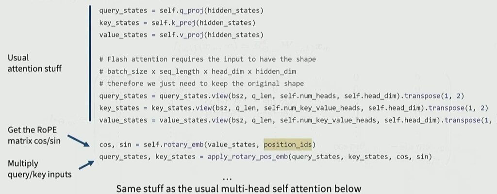
Then you’re going to come up with cosine and sine angles—these are rotation angles telling you how much to rotate different blocks of the query and key. So you take your query and your key, and you’re going to rotate them by the cosines and sines:
cos, sin = self.rotary_emb(value_states, position_ids)
query_states, key_states = apply_rotary_pos_emb( query_states, key_states, cos, sin )
And now you’ve got rotated query and rotated key. That’s going to be what goes into the rest of your attention computation:
# Flash attention requires the input to have the shape
# batch_size x seq_length x head_dim x hidden_dim
query_states = query_states.view(
    bsz, q_len, self.num_heads, self.head_dim).transpose(1, 2)
key_states = key_states.view(bsz, q_len, self.num_key_value_heads, self.head_dim
).transpose(1, 2)
value_states = value_states.view(
    bsz, q_len, self.num_key_value_heads, self.head_dim
).transpose(1, 2)
RoPE Has Won the Position Embedding Battle
One of the things I want to highlight is that RoPE is actually one of the things that it seems like everyone has converged on. Examining all 19 major model papers, basically all of them now use RoPE.
For various different reasons, RoPE has many different algorithms for extrapolating context length, and that’s an important part of modern production language models. But also, it seems to be empirically quite effective, even at fairly small scales and small context lengths. So it’s kind of won out in this position embedding battle.
So you don’t do this at the bottom—you do it whenever you generate your queries and keys. That’s really critical to enforcing this relative positioning information.
8. Feedforward Dimension Scaling
When designing the feedforward network component of transformer architectures, one of the key decisions involves determining the relationship between the feedforward dimension $d_{ff}$ and the model dimension $d_{model}$. This seemingly simple ratio has significant implications for model performance and computational efficiency.
Understanding the Feedforward Dimensions
The feedforward dimension represents the output hidden dimension of your MLP, from which you project back onto \(d_{model}\). In general, these feedforward networks are designed as up-projections, meaning you’ll have more hidden units than there were inputs.
But the critical question remains: how much bigger should this dimension be?
$$\text{FFN}(x) = \max(0, xW_1 + b_1)W_2 + b_2$$
The Standard 4x Rule
The answer has become remarkably standardized across the field. Almost everybody using ReLU-style MLPs picks:
$$d_{ff} = 4 \cdot d_{model}$$
💡 Why 4x?
This 4x ratio has emerged as a strong consensus in the community. While there’s empirical evidence supporting this choice, there’s no fundamental law of nature dictating it. It’s simply a convention that has proven remarkably durable and effective across different architectures and applications.
There are, however, some notable exceptions to this rule. The original T5 paper, for instance, justified picking a much smaller ratio to achieve bigger and more efficient matrix multiplications. The reasoning is that wider matrices enable more parallel computation rather than serial computation, allowing you to spend your FLOPs and parameters in a different way.
While making hidden units bigger would allow more information to pass through, and using more units would provide more serial computation capacity, the wider approach trades some expressive power for potential systems-level performance gains when matrices are sufficiently wide.
GLU Variant Scaling: The 2/3 Rule
The standard 4x ratio we just discussed changes dramatically when working with GLU variants. These architectures scale down by a factor of \(\frac{2}{3}\), which is crucial because it allows you to maintain roughly the same number of parameters as traditional feed-forward networks.
The 8/3 Ratio for GLU
If you scale the GLU variants down by this factor of \(\frac{2}{3}\), you’ll find that the optimal way to achieve this is to set:
$$d_{ff} = \frac{8}{3} d_{model} \approx 2.67 d_{model}$$
You can convince yourself that this parameterization will give you the same number of parameters, and this ratio naturally emerges when you start with the traditional ratio of 4.
When you examine many of the popular models in practice, you’ll find that they actually do follow this rule of thumb quite closely. For instance, PaLM follows this pattern, though models like Mistral and LLaMA are slightly larger than the theoretical 2.6 ratio. These are GLU models, but they don’t strictly adhere to the \(\frac{8}{3}\) rule.
However, if you look at other examples like LLaMA-1, Qwen, DeepSeek, Yi, and T5, they all roughly follow this 2.6-ish rule that emerges from the scaling factor. This represents a very significant difference in architectural design compared to traditional approaches.
T5: The Bold Exception
Speaking of bold exceptions, most large language models tend to have rather boring, conservative hyperparameters. However, there’s one notable exception that stands out for how bold it is: the T5 model by Raffel et al.
🔴 T5’s Extreme Choice
If you look at the 11 billion parameter T5 model, they have a pretty incredible setting:
- Hidden dimension: \(d_{model} = 1024\) (fairly standard)
- Feedforward dimension: \(d_{ff} = 65,536\) (absolutely massive!)
$$\frac{d_{ff}}{d_{model}} = \frac{65,536}{1024} = 64$$
This creates an astounding 64-times multiplier, which is far beyond what most other models attempt!
To put this in perspective, when you compare this to other models, the difference is striking. PaLM uses only about a factor of 4, and most everyone else uses much smaller ratios. Even Gemma 2, which follows somewhat in T5’s footsteps, only goes up to a factor of 8.
💡 The TPU Motivation
The T5 team specifically chose to scale up $d_{ff}$ because modern accelerators like the TPUs they trained on are most efficient for large dense matrix multiplications, exactly like those found in the Transformer’s feed-forward networks.
What’s particularly encouraging about T5’s approach is that it demonstrates these extreme ratios are not just theoretically possible but practically viable. The model turned out to be totally fine despite this unconventional choice!
Empirical Evidence: The Optimal Range
To understand the empirical basis for these design choices, we can turn to Jared Kaplan’s scaling law paper. The researchers explored the \(d_{ff}\) to $d_{model}$ ratio by plotting how much the loss increases as this ratio varies.
A Wide Basin of Optimality
What emerges is a clear sweet spot pattern, with ratios ranging from 1, 2, 3, 4, and extending up to 10 or so, revealing a pretty wide basin where you can pick whatever feed-forward ratio you want and achieve roughly optimal performance.
The empirical evidence shows there’s a basin between 1-10 where this hyperparameter remains near-optimal, and the standard choice of 4 falls right within this sweet spot—it’s not too far off from the optimal choices.
From all this hyperparameter analysis, we can extract some practical guidelines:
Practical Guidelines
- If you’re not using GLU activation: multiply by 4 (\(d_{ff} = 4d_{model}\))
- If you’re using GLU: use roughly 2.66 (\(d_{ff} = 2.66d_{model}\))
These default choices have worked well for nearly all modern language models.
9. Attention Head Configuration
Let’s start by examining the fundamental design choices in multi-head attention architecture. One of the key questions when building transformers is: how do we split up the model dimension across attention heads? The answer to this question has significant implications for both model expressiveness and computational efficiency.
The Canonical Choice: Dimension Splitting
The canonical choice is to maintain a fixed total dimension \(D\) (the hidden dimension) while splitting it evenly across multiple heads. As you add more heads, you simply divide the available dimensions among them rather than keeping each head’s dimension constant.
While you could alternatively maintain the same number of dimensions per head as you scale up—letting the attention mechanism consume more parameters—most successful models follow the dimension-splitting approach.
This doesn’t have to be true: we can have head-dimensions > model-dim / num-heads, and there are 4 matrices \(W^Q, W^K, W^V, W^O\) each of size \((d_{model}, d_{model})\).
Looking at major language models like GPT-3, T5, Lambda, PaLM, and Llama-2, we see they all maintain a ratio of approximately one between model dimension and head allocation. T5 stands out as the notable exception, experimenting with a much larger ratio of 16, but otherwise there’s remarkable consensus in the field. This consistency suggests the approach has proven effective across different model architectures and scales.
💡 Computational Efficiency of Multi-Head Attention
From a computational perspective, computing \(h\) attention heads isn’t significantly more expensive than single-head attention. The process involves:
- Computing \(XQ \in \mathbb{R}^{n \times d}\)
- Reshaping to \(\mathbb{R}^{n \times h \times d/h}\) (same for \(XK\) and \(XV\))
- Transposing to \(\mathbb{R}^{h \times n \times d/h}\)
After transposing, the head axis effectively becomes a batch axis, making the subsequent operations nearly identical with matrices of the same sizes.
However, this conventional wisdom hasn’t gone unchallenged. Notable research by Bhojanapalli and colleagues in 2020 argued against the standard one-to-one ratio, suggesting that as you increase the number of heads, they tend to have progressively lower rank. This raises interesting questions about whether the field’s consensus approach is truly optimal.
Empirical Evidence on Dimension Ratios
Building on those theoretical concerns, let’s look at what the empirical evidence tells us about dimension ratios. When designing transformer architectures, the relationship between dimensions per head becomes crucial for maintaining expressiveness in attention operations.
The Practical Reality
If you have very few dimensions per head, that’s going to start affecting the expressiveness of the attention operation. However, in practice, it doesn’t really seem like we see too many significant low-rank bottlenecks, and most models with a ratio of one seem to do just fine.
This parameter has generally been held constant by most of the models we’ve seen, though there have been papers written against the 1-1 ratio (Bhojanapalli et al 2020).
Aspect Ratio: Deep vs Wide Models
One of the most critical hyperparameters to consider is the aspect ratio—the fundamental question of should my model be deep or wide? How deep and how wide?
Deep vs Wide: The Trade-Off
We can think about deep networks with more and more layers, or we can have wide networks. Generally, if you want one knob to control the width, that would be the hidden dimension of the residual stream, which controls essentially the width of almost all operations at once.
You might think that deeper networks are smarter and more expressive, while wider networks are more efficient.
There is generally a sweet spot of ratios that people have picked, though there have been some outliers. Some of the early models used much smaller ratios, meaning they were much wider than they were deep. However, there’s been a general convergence toward wanting about 128 hidden dimensions per layer, and this approach has been consistently followed by many of the GPT-3 and Llama variant models.
Parallelism Constraints and Aspect Ratio
Now let’s dive deeper into the practical implications of these aspect ratio choices. When designing neural network architectures, aspect ratio considerations play a crucial role in determining the amount of parallelism we can achieve.
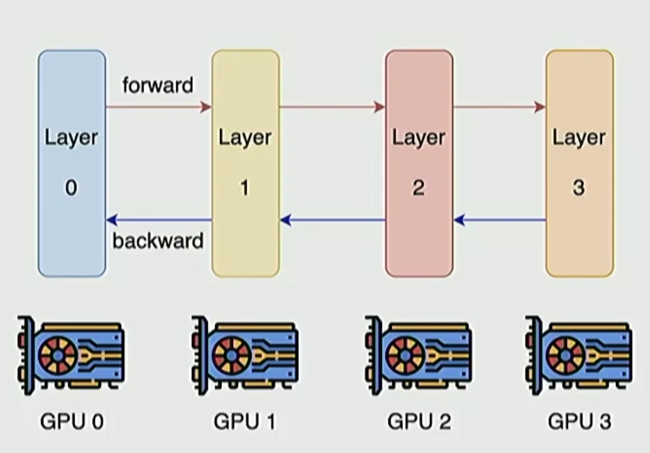
🔴 Pipeline vs Tensor Parallelism
For pipeline parallelism, we typically take different layers and distribute them across different devices or blocks of devices, since we can also parallelize within each layer. This approach places certain constraints on our model design.
Alternatively, for really wide models, we can employ tensor parallelism, where we slice up the matrices and distribute them across GPUs.
These different parallelism paradigms come with distinct constraints: Tensor parallelism requires really fast networking, while pipeline parallelism can tolerate slower networking or higher latency connections. Your networking constraints might therefore drive some of these width versus depth considerations.
The Optimal Aspect Ratio
Setting these practical concerns aside, we can ask more abstractly: what is the impact of aspect ratio on model performance?
Kaplan et al. provide excellent visual evidence showing how aspect ratio impacts performance across three different scales: 50 million, 274 million, and 1.5 billion parameters. The \(x\)-axis shows the aspect ratio, while the \(y\)-axis represents the loss difference in percentage change.
💡 The Sweet Spot Around 100
Remarkably, around the ratio of 100—which aligns with the consensus choice of hyperparameters—we see the minimum across different scales. This finding is backed by large-scale hyperparameter data published by Kaplan et al. and matches our intuition quite well.
A particularly encouraging result is that the optimal aspect ratio doesn’t shift significantly across several orders of magnitude in model size. If this pattern continues to hold, it’s very good news—you can keep training on one fixed aspect ratio as you scale up.
However, there’s an interesting nuance discovered by Tay and others at Google in their study of depth versus width trade-offs. They found that when looking at upstream losses, parameter count is the only thing that matters—deeper models don’t provide additional benefits.
But the story becomes less clear when examining downstream accuracy, such as fine-tuned SuperGLUE performance, where deeper models might actually be better for the same amount of FLOPs.
10. Regularization and Training Stability
As we continue our exploration of training large language models, let’s examine vocabulary size selection, regularization techniques, and the surprising dynamics of weight decay in modern transformer training.
The Trend Toward Larger Vocabularies
There’s been a clear trend toward larger vocabularies in recent years. This shift is largely driven by the deployment of LLMs as real-world services, where they encounter diverse linguistic environments including multiple languages, emojis, and various other modalities that extend beyond traditional text.
Earlier models, particularly those focused on monolingual tasks, typically operated with vocabulary sizes in the 30,000 to 50,000 token range, as we saw with early GPT models and the original LLaMA.
However, multilingual and production systems have shifted dramatically toward the 100,000 to 250,000 token range. This is evident in models like Cohere’s Command R, which emphasizes multilingual capabilities and employs very large vocabulary sizes, as well as GPT-4 and many systems that have adopted the GPT-4 tokenizer, which operate around 100,000 tokens.
💡 Vocabulary Scaling Benefits
Research suggests that as models scale up in size, they can effectively utilize increasingly large vocabularies, making good use of more vocabulary elements. This indicates we might see continued growth in token counts as models become larger and are trained on more extensive datasets.
Regarding multilingual vocabularies, they do contribute to improving performance, but the impact varies by language resource level. For high-resource languages like English, you can get away with smaller vocabularies. However, larger vocabularies become really helpful when dealing with minority or low-resource languages.
The Regularization Paradox
Moving from vocabulary considerations to regularization, we encounter an interesting paradox. When you think about pre-training, it seems like the furthest place from regularization that you could imagine.
Why Regularize During Pre-training?
During pre-training, you typically do just one epoch because you have so much data that you can’t even go through all of it. You’re doing one epoch training, and you’re almost certainly not overfitting the data in that single pass.
So you might think: alright, we don’t need regularization for pre-training—let’s just set your optimizer loose and focus entirely on minimizing loss. These are really good arguments for why you shouldn’t need to regularize.
But then if you look at what people actually do in practice, the story is quite mixed. In the early days, people did use a lot of dropout during pre-training. There’s also been a lot of weight decay that seems to be happening consistently.
🔴 The Evolution of Regularization
These days, many researchers have stopped publishing the precise details of their training hyperparameters, but dropout has sort of gone out of fashion while weight decay has remained something that a lot of people continue to use.
And why is that? It’s really an odd thing to be doing. If you’re training a really large neural network for one pass on SGD with vast amounts of data, why would you use weight decay when you’re doing that? It’s very intuition-violating, at least for me.
Weight Decay: The Surprising Truth
Diving deeper into this weight decay mystery, we discover that the conventional wisdom about weight decay in large language models turns out to be fundamentally wrong. Weight decay isn’t actually controlling overfitting in the way we traditionally understand it.
Weight Decay Doesn’t Control Overfitting
If you examine different amounts of weight decay, they don’t really seem to change the ratio of training loss to validation loss. You can train with different amounts of weight decay—if you train for long enough and control your hyperparameters appropriately, you end up with the same train-to-validation loss gap.
So overfitting? Nothing’s happening here, even with zero weight decay.
What’s actually interesting is that weight decay seems to be interacting in a strange way with the learning rate schedules of the optimizers. When you look at a model trained on constant learning rate and then suddenly decrease the learning rate by $10\times$ or to $0$, you see this drop-off as you decrease the learning rate.
💡 The Learning Rate Interaction
With weight decay, the model’s not training very well at this high learning rate, but when you decrease the learning rate, it’ll very rapidly drop off. When you examine cosine learning rate decay, models with high weight decay start out very slow, but then as they cool down—that is, their learning rate decreases—they very rapidly optimize.
There’s some very complex interaction happening between the optimizer and the weight decay that creates an implicit sort of acceleration near the tail end of training, which ends up giving you better models.
🔴 The Real Purpose of Weight Decay
You don’t use weight decay because you want to regularize the model, which is what it was originally defined for. You’re using weight decay in order to get actually better training losses.
You end up doing that because of the various learning dynamics at the tail end of training as you decrease your learning rates to zero. It’s a very interesting and complex—and in some ways troubling—thing to be doing with language models.
The goal is still to get good training loss—that’s the game we’re playing. The surprising thing about weight decay is that somehow it gets us better training losses. The intuitive thing that would make sense is you do weight decay, it gives you better validation losses, but that’s not what happens. What it’s getting you is better training losses, which are also the same as validation losses.
This phenomenon has been observed in recent research, including interesting observations by Andriushchenko et al. (2023) about LLM weight decay.
Training Stability Best Practices
Now that we’ve explored the nuances of vocabulary size, dropout, and weight decay, let’s synthesize what we know about training stability and best practices.
Consensus Hyperparameters
When it comes to selecting hyperparameters for your model, there are certain choices that have become essentially no-brainers—they’ve been validated and basically everyone uses them:
- Hidden size of the MLP
- Head dimensions of multi-head attention (head_dim × num_heads = $D_{model}$)
- Aspect ratio
- Regularization through weight decay
All of these have fairly good consensus evidence for how to pick them.
Interestingly, dropout has gone out of fashion, and there hasn’t been a deep analysis of why it’s helpful or not—there’s no clear evidence it helps training loss, and as logic would dictate, there’s not really a training overfitting issue with these models that can’t even complete one epoch over the training data.
Modern Stability Innovations
Looking at recent developments, particularly in multimodal architectures, most academic and open work uses what you might call shallow or late fusion of modalities—essentially bolting the vision component onto an existing language model.
However, multimodal models have pioneered some pretty interesting techniques for stabilizing language model training. When you bolt on a new vision piece and retrain, that’s a big shock to the model, requiring careful consideration of how to stabilize the training process.
These innovations have actually seeped back into pure text language model training, and what’s stood out in recent releases has been an emphasis on stability tricks—methods to train models in much more stable ways as they get bigger and train for longer periods.
These stability considerations represent the cutting edge of current training methodology and will likely continue to evolve as models scale to even larger sizes and longer training runs.
Summary
These lecture notes are based on the Stanford Course: Large Language Model from Scratch, Stanford University YouTube.