Highlight: In our previous posts we learned how to implement some simple functions that allow us to load, modify and draw some basic shapes on our input images. Now, when we have a solid foundation, it is time to dive deeper to our first image processing techniques. We should keep in mind these techniques because they are fundamental tools for almost all areas of computer vision. Therefore, a basic understanding of image processing is crucial and after we learn them, we can move on and explore some more complicated areas of OpenCV.

In this post, we’ll cover basic image transformations like image resizing, image translation, image rotation and image flipping. So, let’s start and see how this works in more detail.

Tutorial Overview:

1. Introduction to Affine transformation
2. The Identity matrix
3. How to resize an image?
4. How to translate an image with OpenCV?
5. How to flip an image?
6. How to rotate an image?

1. Introduction to Affine transformation

This paragraph will be a little bit tricky because it contains some mathematics or more specifically some linear algebra. But don’t worry. For more complete overview you can check our post Linear transformations and matrices where everything is explained in more detail.

Let’s start with an affine transform.

In geometry, an affine transformation (Latin affinis – “connected with”) is a function that maps an arbitrary connected space onto itself while preserving the dimension of any affine sub-spaces. So, in simple words, it maps points to points, lines to lines or planes to planes, while preserving the ratio of the lengths of parallel line segments. Since picture is a connected collection of pixels (points) affine transformation represents a segment of digital image processing.

Now, let’s move on. If we want to translate our original image, we need to relocate every pixel in it. To achieve this, we will use a single matrix multiplication. For that, we need to introduce the concept of an augmented matrix or an augmented vector. The technique requires that all vectors are augmented with a number “1” at the end. On the other hand, all matrices are augmented with an extra row of zeros at the bottom, and an extra column on to the right.

This concept of adding one can be a bit puzzling. Hm? One idea why we are using an augmented matrix can be observed by processing a 2D image that lies in a fixed plane in a 3D space. In a following video you can see that this shape is processed while we are keeping a \(z \) axis fixed and equal to 1.

So, we use affine transformations when we need to transform our image. In the following paragraphs, we will see how different affine matrices can scale, resize, flip or rotate images.

2. The identity matrix

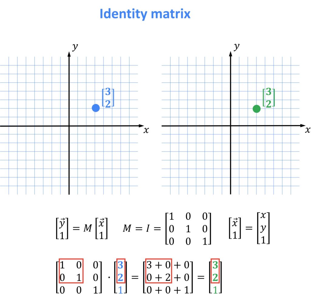
An identity matrix is \(3\times 3 \) matrix with ones on the main diagonal and zeros elsewhere. In a following image we can see a point represented with coordinates \(\begin{bmatrix}3\\2\end{bmatrix} \). This point from a linear algebra perspective can be seen as a vector. Then, we can see what actually happens when we multiply a vector with a matrix. If our matrix is an identity matrix our point will remain at the same location.

3. How to resize an image?

It is very common when we work with images that we have images of different size. Quite often in digital image processing we need to resize our image. We can interpret an operation of resizing using a linear algebra framework. Also, another name that we use is scaling. A scaling matrix can be the following matrix the has no zero elements on the main diagonal. Let’s see how this matrix can remap our original pixels.

So, in this example we relocated every pixel along \(x \) axis. On the other hand, all pixels coordinate values along \(y \) axis remained at the same location. In this example that is the reason why the picture appears stretched along \(x \) axis.

When we are programming with OpenCV in Python, we often need images with specific dimensions. For example, let’s suppose that we want to resize a large image to fit on our computer screen and we need to shrink it. So, how we can do that?

We already learned that a digital image is presented in our computer by a matrix of pixels and each pixel has a specific value. So, if we want to resize our image, we just need to multiply values of our pixels with some scalar. In order to do that we just need to define coordinates of our resized image and apply function cv2.resize(). So, let’s see how it works:

# Necessary imports
import cv2
import numpy as np
# If we are working in Google colab, we are using the function cv2_imshow()
# Otherwise, we will use the function cv2.imshow()
from google.colab.patches import cv2_imshow

# Loading our image
img=cv2.imread("GoT.jpg", 1)
cv2_imshow(img)

Output:

# Resizing the image to 300 x 300
resized = cv2.resize(img, (300, 300))
cv2_imshow(resized)

Output:

O.K. Our image is resized, but do you see the problem? The ratio is not the same. That is why we got this squished image. To fix this problem we need to calculate the aspect ratio of our input image, so that our output image doesn’t appear distorted.

We can easily accomplish our goal. Let’s say that we want to resize width of our original image to 500 pixels, while keeping the same aspect ratio. We can do this in a following way:

# Dimension of our original image
dimensions = img.shape
print(dimensions)

Output:

(549, 969, 3)

# Defining the width and height
h=549
w=969
# Definig aspect ratio of a resized image
ratio = 500.0 / w
# Dimensions of a resized image
dim = (500, int(h * ratio))
# We have obtained a new image that we call resized3
resized_2 = cv2.resize(img, dim)
cv2_imshow(resized_2)

Output:

4. How to translate an image with OpenCV?

When working with multiple images, we often want to move our image from one place to another. Now we will show how to do that. We will transfer the entire content within one image. It is clear that in such a case we will lose some area of the image (this process is particularly useful when, for example, you want to remove an ex-boyfriend or ex-girlfriend from the picture). We call this process a translation of an image.

In order to translate our image, the first thing that we need to do is to create our translation matrix M. This matrix will define the distance and the direction in which we need to shift pixels of our input image. The translation matrix is shown in the following picture.

Now, to get a better understanding lets have a look at the next example.

We can see that pixel \(\begin{bmatrix}3\\2\end{bmatrix} \) now have coordinates \(\begin{bmatrix}7\\-3\end{bmatrix} \). So, a pixel is shifted 4 pixels to the right and 5 pixels down. It is good to remember that positive values of \(t_{x} \) will shift the point to the right and negative to the left. Similarly, positive values of \(t_{y} \) will shift the image up and negative down.

Linear algebra vs image coordinate system. It is good to note that this example is created from the linear algebra perspective and that in image processing our \(y \) axis is going in the opposite direction (down). That is why Python will shift our image in reverse order (down for positive values of \(t_{y} \) and up for negative values).

Our next step is to call a function cv2.warpAffine(). This function transforms the original image using the \(M \) matrix. The first parameter is our original image, the second parameter is the matrix \(M \), and the third parameter establishes the dimensions of our output image. It is important to note that OpenCV expects this matrix to be of floating point type. That is why we define our \(M \) matrix as a floating point array. We can better understand this if we look at following code:

height, width = img.shape[:2]
# Negative values of tx will shift the image to the left
# Positive values will shift the image to the right
# Negative values of ty will shift the image up
# Positive values will shift the image down
M = np.float32([[1, 0, 100], [0, 1, 50]])
translated = cv2.warpAffine(img, M, (width, height))
cv2_imshow(translated)

Output:

5. How to flip an image?

Next, we will learn how to flip an image. This means that we are going to flip our image around \(x \) or \(y \) axis. Moreover, we can even do both operations at the same time. Hay, but don’t worry, it is very simple. We just need to call cv2.flip(). This function is easy, we need to provide only one argument. This argument is a value that will determine around which axes we will flip our image. A value 1 indicates that we are going to flip our image around the y-axis (horizontal flipping). On the other hand, a value 0 indicates that we are going to flip the image around the x-axis (vertical flipping). If we want to flip the image around both axes, we will use a negative value (e.g. -1).

Matrix that we are using to perform this operation in linear algebra is called a reflection matrix. For flipping operations in Python this matrix is not required, but it is good to know how it looks like.

Now, lets continue with our code.

# Flipping the image around y-axis
flipped = cv2.flip(img, 1)
cv2_imshow(flipped)

# Flipping the image around x-axis
flipped = cv2.flip(img, 0)
cv2_imshow(flipped)

# Flipping the image around both axes
flipped = cv2.flip(img, -1)
cv2_imshow(flipped)

This is how all our outputs look like

Output:

6. How to rotate an image?

Now let’s explain how to rotate an image. First, we need an angle \(\theta \) that will represent by how many degrees we are rotating our image. When we perform rotation in linear algebra we always rotate along the center of the coordinate system, However, in OpenCV while processing images we can also rotate our image along arbitrary point which can be defined as an additional parameter of our function. For instance, very often this parameter can be a center of the image and it will be defined in the following way.

In order to calculate the center point, we need height and width of our image. Note that we work with integers when pixels are concerned and therefore we will use “//” division. Then, we can divide each by two to obtain the center point.

Now we need to define our rotation matrix \(M \).

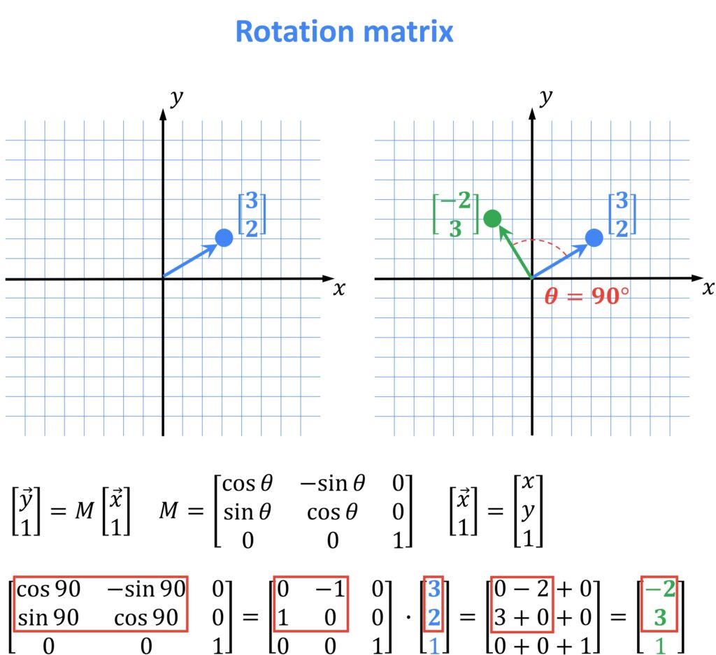
To better comprehend how this matrix works let’s take a look at the next example:

We can see here that our \(\begin{bmatrix}3\\2\end{bmatrix} \) pixel multiplied by \(M \) is now rotated by counterclockwise \(90^{\circ} \).

After defining a rotation matrix \(M \) we need to call cv2.getRotationMatrix2D() function which has few arguments. The first argument is the point around which we want to rotate the image, in our case it will be the center. The second is angle \(\theta \) which determines the value of degrees that we are going to rotate the image by. It is good to remember that if \(\theta \) is positive, our output image will rotate counterclockwise. Similarly, if \(\theta \) is negative the image will rotate clockwise. The third and the last argument is an integer that determines dimensions of our output image. For example, if we put a value 1, our rotated image will have the same dimensions. If we use a value 2 we will get image which is doubled in size.

Finally, we can apply the rotation to our image using cv2.warpAffine()method. We need to specify our rotation matrix \(M \) and the height and the width of our output image. So, lets see how our code looks like.

# Width and height of the image
h, w = img.shape[:2]
# Calculating a center point
# Integer division "//"" ensures that we receive whole numbers
center = (w // 2, h // 2)
# Defining a matrix M and calling
# cv2.getRotationMatrix2D method
M = cv2.getRotationMatrix2D(center, 60, 1.0)
# Applying the rotation to our image using the
# cv2.warpAffine method
rotated = cv2.warpAffine(img, M, (w, h))
cv2_imshow(rotated)

Output:

Summary

In this post, we explained what an Affine transformation of an image is. We have reviewed some common image processing techniques from the Linear Algebra point of view. Also, we learned how to resize, translate, rotate and flip an image. In the next post we will learn how to filter, sharpen and blur our images.

References:

[1] Mastering OpenCV 4 with Python by Alberto Fernández Villán

[2] Practical Python and OpenCV by Adrian Rosebrock