CamCal 004 What does R look like?
Highlights: In this post we will continue working on camera calibration, and we will take a detailed look how does \(R \) look like. If you don’t remember what is \(R \), that is a rotation operator.
Tutorial Overview:
1. Intro
There are two ways to think about this rotation operator. First, we will think in a hard way.
\(_{A}^{B}\textrm{R} \) expresses how each base vector in \(A \) would be expressed in terms of \(B \).

So, the first column of \(_{A}^{B}\textrm{R} \) is the component of \(i_A \) expressed in terms of how much it has in the \(i \) direction in \(B \), in \(j \) direction in \(B \) and in \(k \) direction in \(B \). You can think of it as a dot product between \(i_A \) and each of the components of \(B \) ( \(i_B \), \(j_B \) and \(k_B \)). Likewise each of the following columns are created in that way.
$$_{A}^{B}\textrm{R} = \begin{bmatrix} i_A .i_B & j_A .i_B & k_A .i_B \\ i_A .j_B & j_A .j_B & k_A .j_B \\ i_A .k_B & j_A .k_B & k_A .k_B \end{bmatrix} = \begin{bmatrix} { }^{B}\textrm{i}{A} &{ }^{B}\textrm{j}{A} &{ }^{B}\textrm{k}_{A}\end{bmatrix}$$
One way of thinking of this is that columns of \(_{A}^{B}\textrm{R} \) are \(i\) vector of \(A\) expressed in \(B \) coordinate frame, then the \(j\) vector of \(A\) in \(B \) coordinate and \(k\) vector of \(A\) expressed in \(B \) coordiante frame.
Columns of the rotation matrix are the axes of the frame \(A \) expressed in frame \(B \).
2. Example: Rotation About Z-Axis
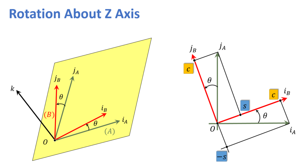
Let’s take a few simple examples. Here we have two frames.

Above we have two frames, and we can tell that rotation of \(A \) to \(B \) is just about \(z \) axis. So, on the image in the right we are looking down on the \(z \) – axis. We can talk about the rotation of angle \(\theta \) about the origin when we are doing \(x -y \). It is something that looks like this:
$$ R(\theta ) = \begin{bmatrix} cos( \theta) & -sin(\theta ) & 0 \\ sin( \theta ) & cos(\theta ) & 0 \\ 0 & 0& 0 \end{bmatrix} $$
The point is that this matrix is just for rotating the \(x \) and \(y \) keeping the \(z \) constant.
So, if we want to get the arbitrary orientation basically what we can do is a series of rotations to feed things where we want them. It turns out that there are many standards about how to do that:
- Most of us know about Euler angels. This rule means that we rotate about \(Z \), rotate about new \(X \) and rotate about new \(Z \).
- Heading, pitch roll: world \(Z \), new \(X \), new \(Y \)
- Roll, pitch and yaw
- Azimuth, elevation, roll
Basically there are these \(3 \) rotation about \(X, Y \) and \(Z \) and the order matters. But we won’t worry that much in fact, not at all about getting that order.
So, here are the three rotation matrices are written as functions of their angles. There are rotation about \(X \), about \(Y \) and rotation about \(Z \).
$$ R_{X}(\phi) = \begin{bmatrix} 1 & 0 & 0 \\ 0& cos(\phi) & -sin(\phi) \\ 0 & sin(\phi)& cos(\phi) \end{bmatrix} $$
$$ R_{Z}(\theta ) = \begin{bmatrix} cos( \theta ) & -sin(\theta ) & 0 \\ sin( \theta ) & cos(\theta ) & 0 \\ 0 & 0& 0 \end{bmatrix} $$
$$ R_{Y}(k) = \begin{bmatrix} cos( k) & 0 & -sin(k) \\ 0 & 1 & 0 \\ sin(k) & 0& cos(k) \end{bmatrix} $$
The idea is that you can rotate about each of these axes.
Whether you premultiply or post-multiply that’s the issue. So whether we do the \(X_1 \) and then the \(X_2 \) or the other way it depends on whether we are rotating on the new frame or the old frame. Then, is \(\theta \) positive or negative? So, you have to worry about these things really well.
How about an easier way?
3. Rotation in Homogeneous Coordinates
Once again to the rescue, homogenous coordinates will arrive. Using homogenous coordinates, rotation can be expressed as matrix multiplication. We are just going to assume that we have a rotation matrix. The following equation makes \(_{}^{B}\textrm{P} \) the rotated version of \(_{}^{A}\textrm{P} \) .
\( _{}^{B}\textrm{P} = _{A}^{B}\textrm{R} \enspace _{}^{A}\textrm{P} \)
$$ \begin{bmatrix} _{}^{B}\textrm{P} \\ 1 \end{bmatrix} =
\begin{bmatrix} _{A}^{B}\textrm{R} & \textbf{0} \\ \textbf{0} ^T & 1 \end{bmatrix} \begin{bmatrix} _{}^{A}\textrm{P} \\ 1 \end{bmatrix} $$
And now instead of having an offset on the right, we have the roration matrix \( _{A}^{B}\textrm{R } \) which is \(3 \times 3 \) dimensional. The zero matrix, \(\textbf{0} \) is \(3 \times 1 \) dimensional.
To remind, unlike translation , rotation is not commutative.
4. Rigid Transformation
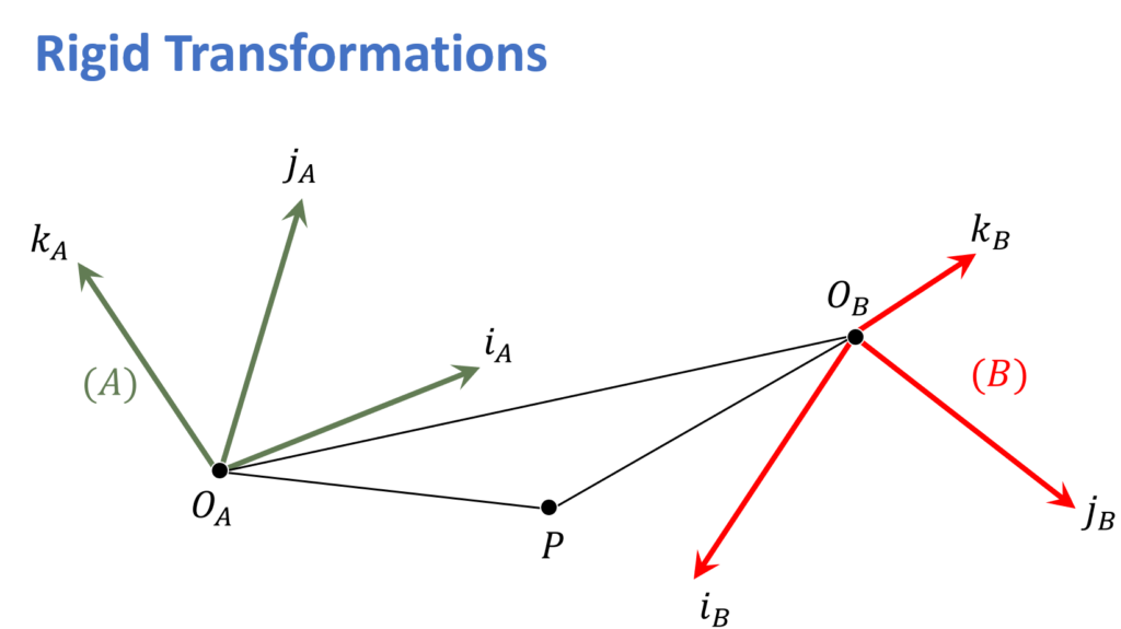
So, now we can do the total Rigid transformation. The total rigid transformation is:
$$ _{}^{B}\textrm{P} = _{A}^{B}\textrm{R} _{}^{A}\textrm{P} + _{}^{B}\textrm{O}_{A} $$
If we have a point in \(A \) system, we first have to rotate it to have it in the \(B \) system and then we have to offset it by whatever the offset in \(A \) system of \(B\) system is. That is what following equation says. Using homogenous coordinates we can do it all in one step.

Here we have a Rigid transformation
$$ \begin{bmatrix} _{}^{B}\textrm{P} \\ 1 \end{bmatrix}
= \begin{bmatrix} 1 & _{}^{B}\textrm{O}_{A} \\ \textbf{0}^T &1 \end{bmatrix} \enspace \begin{bmatrix} _{A}^{B}\textrm{R} & 0 \\ \textbf{0}^T &1 \end{bmatrix} \enspace \begin{bmatrix} _{}^{A}\textrm{P} \\ 1 \end{bmatrix}
= \begin{bmatrix} _{A}^{B}\textrm{R} & 0 \\ 0^T & 1 \end{bmatrix} \begin{bmatrix} _{}^{A}\textrm{P} \\ 1 \end{bmatrix} $$
The first matrix in the equation above is for the translation, and the second one is for the rotation.
Using homogenous transformation or homogenous coordinates we can do all in one step. So, here we have a Rigid transformation. Our total rotation matrix is \(4\times 4 \) dimensional and it performs both translation and rotation.
So, we get \(P \) expressed in the \(B\) frame when we multiply the rotation matrix with the \(P \) expressed in the \(A \) frame. So the previous equation we can write as a transformation from \(A \) to \(B \)
$$ \begin{bmatrix} _{}^{B}\textrm{P} \\ 1 \end{bmatrix} = \begin{bmatrix} _{A}^{B}\textrm{R} & _{}^{B}\textrm{O}_{A} \\ \textbf{0}^T &1 \end{bmatrix} \begin{bmatrix} _{}^{A}\textrm{P} \\ 1 \end{bmatrix} = _{A}^{B}\textrm{T}
\begin{bmatrix} _{}^{A}\textrm{P} \\ 1 \end{bmatrix} $$
Suppose that we want to go from \(B\) to \(A \):
$$ \begin{bmatrix} _{}^{A}\textrm{P} \\ 1 \end{bmatrix} = _{B}^{A}\textrm{T}
\begin{bmatrix} _{}^{B}\textrm{P} \\ 1 \end{bmatrix} = _{A}^{B}\textrm{T}^{-1}
\begin{bmatrix} _{}^{B}\textrm{P} \\ 1 \end{bmatrix} $$
This transformation brings back the information from the \(B \) frame back to the \(A \) frame.
The idea is that our transformation matrices are homogenous \(4\times 4 \) matrices that are invertible. So, once we have one that goes from the camera to the real world we can go “from world to camera” or the other way around.
This invertabillity of the homogenous coordinates is very powerfull and used all the time.
Summary:
To summarize, here we have looked in a little more detail how the rotation operator looks like, and how we can do the rotation and translation using it. Next thing, we can use this to take a deeper look at rotation and translation, both in non-homogeneous and homogeneous coordinates. We will talk about this in the next post.