#009 The Singular Value Decomposition(SVD) – illustrated in Python

Highlight: In this post, we will talk about the Singular Value Decomposition (SVD). We will see that is the continuation of the Linear Algebra post about eigenvectors and eigenvalues. Well, it is probably one of the most important algorithms in Linear Algebra, math, and engineering. Applications are immense, starting from Image processing, Computer vision, up to industrial applications, such as Google rank algorithm. O.K., you probably heard about SVD already. So, let’s start!
Tutorial Overview:
- What is Singular Value Decomposition?
- Eigenvectors for the SVD
- SVD – a more formal definition
- Implementation of SVD in Python
1. What is Singular Value Decomposition?
Let’s briefly discuss what Singular Value Decomposition (SVD) algorithm is all about. Here, we say that SVD is a matrix decomposition algorithm. It will create a set of new matrices, and when we multiply back these matrices, we will reconstruct the original matrix. So far, so good.
Now, we will introduce the motivation behind the idea of decomposition. In some cases, matrices have a particular structure. If there is a regular or simple structure in the matrix, then the decomposition application would be more beneficial and powerful. Let us have a look at the following introductory example.
Example 1.1
Imagine that we need to send the following matrix. It is a very simple one having all pixel values equal.
$$ A= \begin{bmatrix}1 &1 & 1 & 1 & 1 & 1\\ 1 & 1 & 1 & 1 & 1 & 1\\ 1 & 1 & 1 & 1 & 1 & 1\\ 1 & 1 & 1 & 1 & 1 & 1\\ 1 & 1 & 1 & 1 & 1 & 1\\ 1 & 1 & 1 & 1 & 1 & 1\end{bmatrix} $$
Intuitively, we see that it is possible to compress this matrix. There are many possible ways, but we will do this using an outer vector product. If this term is not familiar to you, just think that it is a regular matrix multiplication of two matrices. So, instead the original \(36 \) elements of a matrix \(A \), we can send two vectors of \(6 \) elements, thereby sending \(12 \) elements in total.
$$ A = \begin{bmatrix}1\\ 1\\ 1\\ 1\\ 1\\ 1\end{bmatrix}\begin{bmatrix}1 & 1 & 1 & 1 & 1 & 1\end{bmatrix} $$
This matrix can be regarded as an image that’s very simple \((6\times 6) \) with all white pixels. So far so good, and I do know that you are not impressed. But, let’s proceed. Let’s suppose that we have now an Italian flag.
Example 1.2 – Italian flag
Again, our new flag is a rather simple structure, but slightly more complex. It has three vertical stripes and it can be illustrated as follows:

$$ A= \begin{bmatrix}g &g & w & w & r & r\\ g &g & w & w & r & r\\ g &g & w & w & r & r\\ g &g & w & w & r & r\\ g &g & w & w & r & r\\ g &g & w & w & r & r\end{bmatrix} $$
Now, we can apply a similar idea as before and write it in the form of an outer vector product (i.e., column vector times row vector). A column vector is again a very simple one (all ones), whereas the row vector represents different color values. Again, we have succeeded to simplify our original matrix representation.
$$ A= \begin{bmatrix}1\\ 1\\ 1\\ 1\\ 1\\ 1\end{bmatrix}\begin{bmatrix}g & g & w & w & r & r\end{bmatrix} $$
This was a more complex example and still, we were able to compress it in a very nice way, where we have a column vector of ones and a row vector to store colors. These are all very special cases of image representations, but can we do something a little bit better? Let’s see. One idea is that we can continue applying this trick where we have this column-row vector multiplication. We can apply it to a very simple matrix in the next example. However, note that although a matrix is simple, we won’t be able to represent the whole matrix with just one pair of column-row vectors as you will see.
Example 1.3 – Embedded square
$$ A= \begin{bmatrix}1 & 0\\ 1 & 1\end{bmatrix} $$
One way to decompose a matrix like this one is to try to decompose it using a row-column multiplication. Here, we can see that we cannot do this with only one pair of a column – row vector, but now we need to use more terms. The reason for this is that this matrix has a rank \(2 \).
We can proceed in the following manner. We take our column vector of ones and multiply it by the row vector of ones. This gives us a \(2\times 2 \) matrix which consist of ones. Then, we subtract from this result the matrix multiplication of the column vector \(\begin{bmatrix}1\\0\end{bmatrix} \) and row vector \(\begin{bmatrix}0, & 1\end{bmatrix} \).
$$ A= \begin{bmatrix}1\\1\end{bmatrix}\begin{bmatrix}1 & 1\end{bmatrix}-\begin{bmatrix}1\\0\end{bmatrix}\begin{bmatrix}0 & 1\end{bmatrix} $$
That’s how we decompose our matrix into a summation (or subtraction) of two terms. Each of the terms has the following structure: column times row multiplication.
So, in the previous examples, we have decomposed our original matrices. Indeed, these were straightforward approaches, and we just used them as intuitive introductory examples.
You may ask: haven’t we said to perform a decomposition into product terms? Yes, a product of matrices. Here, we indeed used summation terms, but we will show how we can pack everything together into special matrices so that our original proposition holds. In the further text, it is essential to distinguish vectors and matrices.
What is actually Singular Value Decomposition doing?
The SVD is decomposing our matrix \(A \) into a set of vectors \(v \) and \(u \), and one diagonal matrix (which we will introduce soon). We will have column vectors, row vectors, and scalars that will be used for multiplication. That’s actually Singular Value Decomposition, where we decompose a matrix into terms.
In case that we have a rank = \(2 \), we would be able to decompose our matrix into:
$$ u_{1}v_{1}^{T}+u_{2}v_{2}^{T} $$
And in case that rank = \(1 \), the result should look like:
$$ u_{1}v_{1}^{T} $$
A slightly more complex decomposition would be to add scalars (\(\sigma \) – sigma) which will be stored in a diagonal matrix. Our basic decomposition for a rank-\(2 \) matrix \(2 \):
$$ A= \sigma _{1} u_{1}v_{1}^{T}+\sigma _{2} u_{2}v_{2}^{T} $$
One obvious thing here is that actually we can treat these sigma values as weighting coefficients. Later, we will store them in a diagonal matrix.
2. Eigenvectors for the SVD
We have realized that the matrix \(A \) can be decomposed into vectors \(u \) and \(v \). Still, we need to provide more ideas on how we are going to do this for every matrix. An SVD will be based on the following idea.
If we calculate the eigenvectors \(u \) of a matrix \(AA^{T} \) and the eigenvectors \(v \) of \(A^{T}A \) we would be able to decompose our matrix \(A \) into these vectors.
- The \(u \)s from the SVD will be the left singular vectors and they are unit vectors of \(AA^{T} \)
- The \(v \)s will be right singular vectors and unit vectors of \(A^{T}A \)
- The \(\sigma \)s are the singular values. They are square roots of eigenvalues of \(AA^{T} \) and \(A^{T}A \) and these values are equal
We can write the formulas related to eigenvectors \(u \) in the following way:
$$ AA^{T}u_{i}= \sigma _{i}^{2}u_{i} $$
Example 2.1
Now, let’s see how this looks like in the following example:
The \(u \) vectors are going to be the eigenvectors of \(AA^{T} \).
$$ AA^{T}= \begin{bmatrix}1 & 0\\ 1& 1\end{bmatrix}\begin{bmatrix}1 & 1\\ 0& 1\end{bmatrix}= \begin{bmatrix}1 & 1\\ 1& 2\end{bmatrix} $$
The \(v \) vectors are going to be the eigenvectors of \(A^{T}A \).
$$ A^{T}A= \begin{bmatrix}1 & 1\\ 0& 1\end{bmatrix}\begin{bmatrix}1 & 0\\ 1& 1\end{bmatrix}= \begin{bmatrix}2 & 1\\ 1& 1\end{bmatrix} $$
Their determinants are \(1 \) and their traces are \(3 \).
$$ det\begin{bmatrix}1-\lambda & 1\\1 & 2-\lambda\end{bmatrix}= \lambda ^{2}-3\lambda +1= 0 $$
Which gives us:
$$ \lambda_{1} = \frac{3+\sqrt{5}}{2} $$
$$ \lambda_{2} = \frac{3-\sqrt{5}}{2} $$
If we calculate \(\sqrt{ \lambda_{1} } \) and \(\sqrt{ \lambda_{2} } \) we get:
$$ \sigma _{1} = \frac{\sqrt{5}+1}{2} $$
$$ \sigma_{2} = \frac{\sqrt{5}-1}{2} $$
What we can do now is to continue forming our \(u_{1} \), \(u_{2} \) and \(v_{1} \), \(v_{2} \) vectors.
\(u_{1}=\left[\begin{array}{l}1 \\\sigma_{1}\end{array}\right] \) ; \({u}_{2}=\left[\begin{array}{c}\sigma_{1} \\-1\end{array}\right] \)
\({v}_{1}=\left[\begin{array}{c}\sigma_{1} \\1\end{array}\right] \) ; \(v_{2}=\left[\begin{array}{l}1 \\-\sigma_{1}\end{array}\right] \)
These values are all divided by:
$$ \sqrt{1+\sigma _{1}^{2}} $$
Now we are able to write how the decomposition of \(A \) will look like:
$$ A= \begin{bmatrix}u_{_{1}} & u_{2}\end{bmatrix}\begin{bmatrix}\sigma _{1} & \\ & \sigma _{2}\end{bmatrix}\begin{bmatrix}v_{1}^{T}\\ v_{2}^{T}\end{bmatrix} $$
$$ Av= A\begin{bmatrix}v_{1} & v_{2}\end{bmatrix}= \begin{bmatrix}\sigma _{1}u_{1} & \sigma _{2}u_{2}\end{bmatrix} $$
If we continue our story about SVD we will see that one way to write this is the following:
$$ Av_{1}= \sigma _{1}u_{1} $$
Using all this we can see that we can decompose our matrix into the following \(3 \) matrices:
$$ A= U\Sigma V^{T} $$
This was just another way to write \(A \) where \(u \) is a column vector, \(v \) transposed is a row vector and \(\sigma_{1} \) is a singular value with the largest absolute value.
Example 2.2
Let’s have a look at the another example. We will find \(U \), \(\Sigma \) and \(V \) for \(A= \begin{bmatrix}3 & 0\\4 & 5\end{bmatrix} \). Without proving this, we will say that the rank is equal to \(2 \). It will have two singular values \(\sigma_{1} \) and \(\sigma_{2} \). We will be able to calculate these as eigenvalues in a simple way. We will see that \(\sigma_{1} \) is larger than \(\lambda_{max}= 5 \) , and that \(\sigma_{2} \) is smaller than \(\lambda_{min}= 3 \).
First, let’s calculate \(AA^{T} \) and \(A^{T}A \).
$$ A^{T}A = \begin{bmatrix}25 &20 \\ 20 & 25\end{bmatrix} $$
$$ AA^{T} = \begin{bmatrix}9 & 12 \\ 12 & 41\end{bmatrix} $$
Their eigenvalues will be the square roots of \(\sigma _{1}^{2}= 45 \) and \(\sigma _{2}^{2}= 5 \). Their square roots are:
$$ \sigma _{1}= \sqrt{45} $$
$$ \sigma _{2}= \sqrt{5} $$
Basically, we can see that we can also get eigenvectors for these singular values and we see that they are:
For \(v_{1} \):
$$ \begin{bmatrix}1\\1\end{bmatrix} $$
For \(v_{2} \):
$$ \begin{bmatrix}-1\\1\end{bmatrix} $$
$$ \left[\begin{array}{cc}25 & 20 \\20 & 25\end{array}\right]\left[\begin{array}{l}1 \\1\end{array}\right]=45\left[\begin{array}{l}1 \\1\end{array}\right] $$
$$ \left[\begin{array}{cc}25 & 20 \\20 & 25\end{array}\right]\left[\begin{array}{l}-1 \\1\end{array}\right]=5\left[\begin{array}{l}-1 \\1\end{array}\right] $$
Then, \(v_{1} \) and \(v_{2} \) are the orthogonal eigenvectors re-scaled to length \(1 \) and, therefore, divided by \(\sqrt{2} \).
Right singular vectors:
$$ v_{1}= \frac{1}{\sqrt{2}}\begin{bmatrix}1\\1\end{bmatrix} $$
$$ v_{2}= \frac{1}{\sqrt{2}}\begin{bmatrix}-1\\1\end{bmatrix} $$
Left singular vectors:
$$ u_{i}= \frac{Av_{i}}{\sigma _{i}} $$
We can now calculate \(Av_{1} \) and \(Av_{2} \) which are \(\sigma _{1}u_{1}= \sqrt{45} u_{1} \) and \(\sigma _{2}u_{2}= \sqrt{5} u_{2} \)
$$ Av_{1}= \frac{3}{\sqrt{2}}\begin{bmatrix}1\\3\end{bmatrix}= \sqrt{45}\frac{1}{\sqrt{10}}\begin{bmatrix}1\\3\end{bmatrix}= \sigma _{1}u_{1} $$
$$ Av_{2}= \frac{1}{\sqrt{2}}\begin{bmatrix}-3\\1\end{bmatrix}= \sqrt{5}\frac{1}{\sqrt{10}}\begin{bmatrix}-3\\1\end{bmatrix}= \sigma _{2}u_{2} $$
We can now see that the Singular Value Decomposition of \(A \) is \(U \) times \(\Sigma \) times \(V^{T} \).
$$ U= \frac{1}{\sqrt{10}}\begin{bmatrix}1 & -3\\ 3 & 1\end{bmatrix} $$
$$ \Sigma = \begin{bmatrix}\sqrt{45} & \\ & \sqrt{5}\end{bmatrix} $$
$$ V= \frac{1}{\sqrt{2}}\begin{bmatrix}1 & -1\\1 & 1\end{bmatrix} $$
If we want to check if our calculations were correct, we can do that in the following way:
$$ \sigma _{1} u_{1}v_{1}^{T}+\sigma _{2} u_{2}v_{2}^{T}= \frac{\sqrt{45}}{\sqrt{20}}\begin{bmatrix}1 & 1\\ 3 & 3\end{bmatrix} +\frac{\sqrt{5}}{\sqrt{20}}\begin{bmatrix}3 & -3\\-1 & 1\end{bmatrix}= \begin{bmatrix}3 & 0\\ 4 & 5\end{bmatrix}= A $$
To summarize ideas about SVD, we can say that SVD factors \(A \) into a product of three matrices (\(U\Sigma V^{T} \)), where \(r \) are singular values sorted in a decreasing order \(\sigma_{1}\geq …\geq \sigma_{r}> 0 \). These singular values are nonzero eigenvalues of \(AA^{T} \) and \(A^{T}A \). The eigenvectors of \(AA^{T} \) and \(A^{T}A \) will be unit and orthonormal vectors both in \(U \) and \(V \). Hence, they will be able to diagonalize the matrix in the following form:
$$ Av_{i}= \sigma _{i}u_{i} $$ for $$ i\leq r $$
$$ AV= U\Sigma $$
$$ A= U\Sigma V^{T} $$
3. SVD – a more formal definition
We have already learned that SVD creates a set of new matrices, and when we multiply them, we get the original matrix. We will start again with the matrix \(A \) that will be composed of column vectors. As we have explained at the beginning of this tutorial, the idea of the singular value decomposition is to decompose this matrix into a product of three terms. These three terms will be matrices \(U \), \(\Sigma \) and \(V \). So, we are taking matrix \(A \) and representing it as a product of \(U \), \(\Sigma \) and \(V \).

An important thing to remember here is that the matrix \(A \) can have \(m \) columns or column vectors whose length is \(n \). It means that \(A \) is of dimension \(n \) times \(m \). Then, we will have a matrix \(U \). The dimensions of \(U \) will be \(n \) times \(n \). Next, the dimensions of \(\Sigma \) will be \(n \) times \(m \), whereas the dimensions of \(V \) will be \(m \) times \(m \).
$$ dim\left \{ A \right \} = n\times m $$
$$ dim\left \{ U \right \} = n\times n $$
$$ dim\left \{ \Sigma \right \} = n\times m $$
$$ dim\left \{ V \right \} = m\times m $$
One interpretation of columns in matrix \(A \) is that we can have images instead of numerical values. For instance, the images of aligned faces can be stored as columns. In this case, the images are first vectorized (e.g. np.reshape(-1,1)) and stored as columns. On the other hand, it is interesting to say that \(U \) matrix will have similar columns that correspond to the columns in \(A \). It means that \(U \) can be observed as a factor representing the basis of our data. We call these “vector faces” the eigenfaces similarly to the eigenvectors. We can use eigenfaces for face representation, which is an essential method used for face analysis in image processing and computer vision.

It is important to note that \(U \) and \(V \) are so called the unitary matrices. It means that once we multiply \(U \) with \(U^{T} \) and \(V \) with \(V^{T} \), we will obtain identity matrices. In the first case, \(U \) will be \(n\times n \) identity matrix and in the second case, for \(V \) matrix, it will be an identity matrix \(m\times m \).
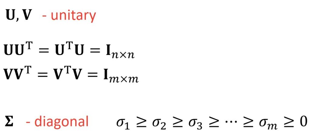
The other important thing to note is that \(\Sigma \) is diagonal matrix. Do note the fact that \(\sigma _{1} \) is larger than \(\sigma _{2} \) and that it is decreasingly ordered. This means that corresponding first columns \(u _{1} \), \(v _{1} \) and \(\sigma _{1} \) are somehow more important factors than the second column, and second column is more important than the third column and so on until the last column. This comes from the idea that \(\sigma _{1} \) will have the largest absolute value from all other \(\sigma \) values in a matrix \(\Sigma \).
Next, we can represent our product of three matrices as a summation of outer product vectors \(u _{1} \) times \(v_{1}^{T} \) times \(\sigma _{1} \). If we have m such terms in the summation, we can often truncate it because \(\sigma \) values are decaying and usually we just keep a lower number of the summation terms. It is important to say that if we use m summation terms, we can perfectly reconstruct our matrix so that the identity holds. On the other hand, if we use just r such terms, it will be a rank-r approximation. The term rank-r refers to r terms of a column-row multiplication (or outer vector product).

How to compute these matrices?
Now we will go more into details of how we can compute matrices \(U \), \(\Sigma \) and \(V \). We will do this from the aspect of correlation and the following matrix is known as a correlation matrix of \(A \). Every element of this matrix is a simple inner product of columns of matrix \(A \).
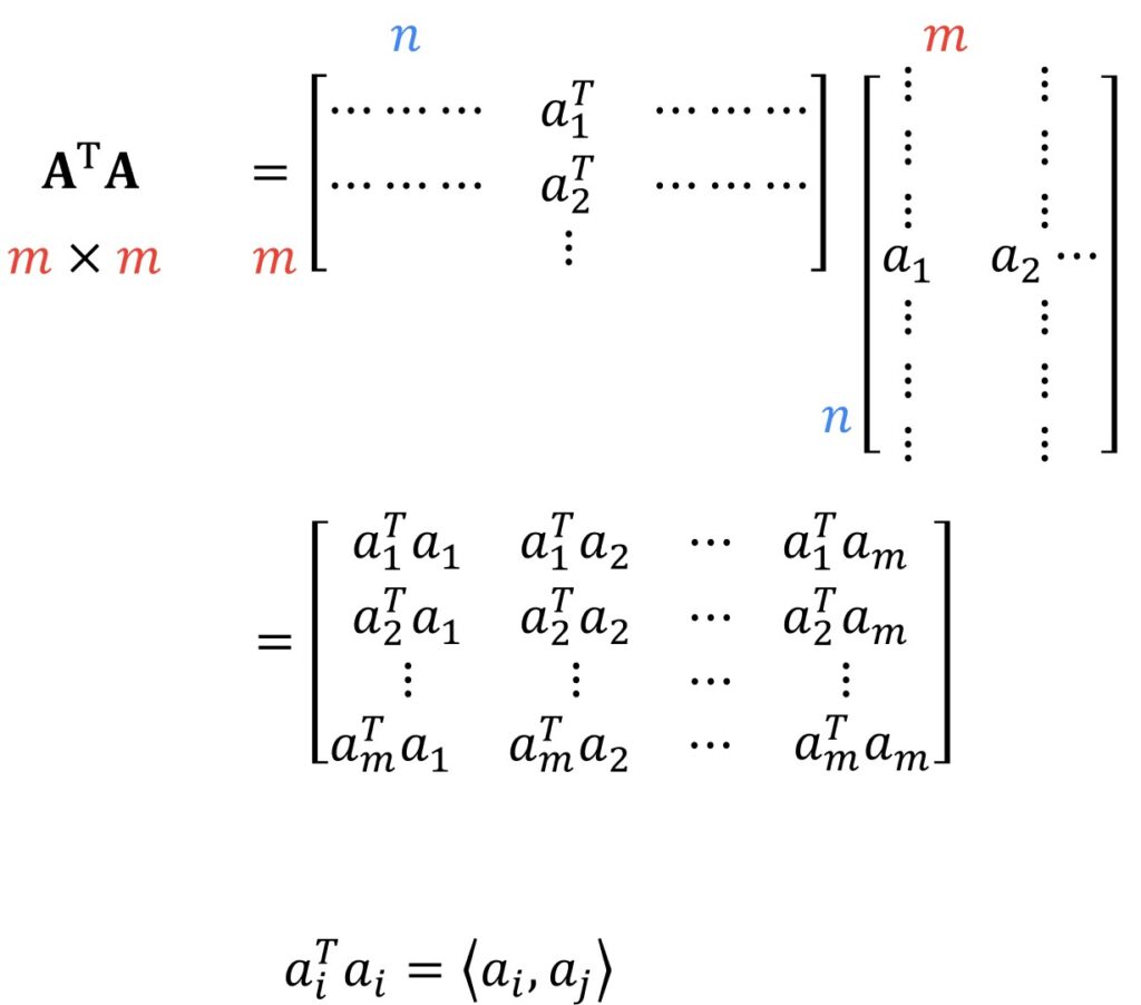
We can interpret this product \(a_{i} \) times \(a_{j} \) as the inner product of the faces of two persons. In case when two persons are similar, we will have a large value. On the other hand, if they are totally uncorrelated, we will get a value near 0. This is something that we know as the property of vectors.
In addition, note that this matrix is symmetric and positive semi-definite. This is due to the commutative property of the inner product. Hence, eigenvalues will be positive, so \(\Sigma \) values will be positive values as well.

Note that the transpose of \(\Sigma \) is \(\sigma \), as it is a diagonal matrix. Also, we can apply the same principle for A * A^T transposed and we will get the following equation. Also, it is important to remember that \(\Sigma \) is the same as the \(\Sigma \) matrix.

4. Implementation of SVD in Python
Singular Value Decomposition
Let us see how we can implement all this theory in Python code. First, we will import the necessary libraries.
#import libraries
import numpy as np
import matplotlib.pyplot as plt
import cv2
We will define a matrix that has a very simple structure.
A = np.ones((6, 6))
A[:,:2] = A[:,:2]*2
A[:,2:4] = A[:,2:4]*3
A[:,4:] = A[:,4:]*4

print(A)
[[2. 2. 3. 3. 4. 4.]
[2. 2. 3. 3. 4. 4.]
[2. 2. 3. 3. 4. 4.]
[2. 2. 3. 3. 4. 4.]
[2. 2. 3. 3. 4. 4.]
[2. 2. 3. 3. 4. 4.]]
We will also define a color map for our example.
our_map = 'hot'
#our_map = 'gray'
Now, let’s apply an SVD. Then, we create a full matrix from the diagonal elements.
U, S, VT = np.linalg.svd(A)
S = np.diag(S)
Next, we will define a helper function draw_svd that we will use to draw the original matrix \(A \) and matrices \(U \), \(\Sigma \) and \(V^{T} \).
def draw_svd(A,U, S, VT, our_map):
  plt.subplot(221 )
  plt.title('Original matrix')
  plt.imshow(A, cmap =our_map)
  plt.axis('off')
  plt.subplot(222)
  plt.title('U  matrix')
  plt.imshow(U, cmap =our_map)
  plt.axis('off')
  plt.subplot(223)
  plt.title('Sigma matrix')
  plt.imshow(S, cmap =our_map)
  plt.axis('off')
  plt.subplot(224)
  plt.title('V matrix')
  plt.imshow(VT, cmap =our_map)
  plt.axis('off')
In case that the diagonal sigma values are too small, for numerical/esthetic purposes, we will remove the corresponding very small \(u \), \(v \) elements. For instance, if a singular value is 1e-08 it will not affect the reconstruction, so we set these small values to zeros.
def truncate_u_v(S, U, VT):
  threshold = 0.001
  s = np.diag(S)
  index = s < threshold

  U[:,index] = 0
  VT[index,:]=0
  return U, VT
U, VT = truncate_u_v(S, U, VT)
draw_svd(A, U, S, VT, our_map) Output:
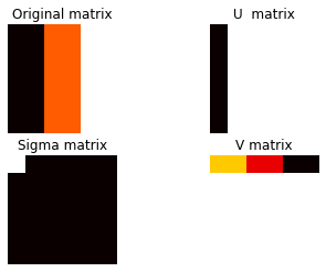
We will use an rank-r approximation (here r=1), and this determines how many summation terms we have:
\(U_{i} \) * \(\Sigma_{i} \) * \(V^{T}_{i} \)
This is also known as a rank-1 approximation.
Let’s see how the \(U, \Sigma \) and \(V^{T} \) look like.
r = 1
A0_r = np.matmul(U[:,:r] , S[:r,:r])
A0_r = np.matmul (A0_r , VT[:r,:])
plt.imshow(A0_r, cmap =  our_map)
plt.axis('off')
For this example, we have seen earlier that the flag can be represented as a rank-1 approximation. In the \(\Sigma \) matrix the first upper element is the only non-zero element. In addition, note that the matrices \(U \) and \(V \), are normalized so that their L2 norm is equal to 1. The \(V \) matrix has one row whose elements determine the different color values.
Now, let’s solve a numerical example of our \(2\times2 \) matrix from the introductory part. Later, we can compare the Python obtained values with the values that we have already calculated.
A = [[1, 0], [1, 1]]
U, S, VT = np.linalg.svd(A)
S = np.diag(S)

print(f"U {U}\nS {S}\nVT {VT}")
Output:
U [[-0.52573111 -0.85065081]
 [-0.85065081  0.52573111]]
S [[1.61803399 0.        ]
 [0.         0.61803399]]
VT [[-0.85065081 -0.52573111]
 [-0.52573111  0.85065081]]
Next, we can show an example where we have images of faces stored as column vectors. One such dataset can be located in the sklearn library – Olivetti faces. In this dataset, the images are already vectorized and stored as columns (64 x 64=4096).
from sklearn.datasets import fetch_olivetti_faces
face = fetch_olivetti_faces()

X = face.data
# The images are of size 64 x 64
X.shape
Output:
(400, 4096)
Here, we are going to take just the first image for this example. Note that this is still not the eigenfaces example. We will explore this in other posts.
faces = X[0,:].reshape((64,64))The next step is to decompose this face and draw the \(U, \Sigma \) and \(V^{T} \) as well as the image we are decomposing.
# we decompose the image of a face
U, S, VT = np.linalg.svd(faces)
S = np.diag(S)
faces = faces.astype('float')
#U, VT = truncate_u_v(S, U, VT)
draw_svd(faces, U, S, VT, 'gray')
Output:
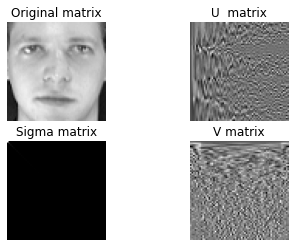
We can plot the singular value or the \(\Sigma \) and we can see that only the first 30 elements have significant values.
diag_elem = np.diag(S)
plt.stem(diag_elem[1:])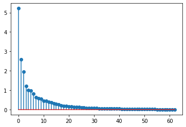
Now comes the interesting part, the reconstruction. We will use the rank-r approximation. The code below will save 100 images which we will add all together to get a GIF of the reconstructions while increasing the r-value. The animation shows how much every successive rank-r approximation contributes to the reconstruction of the image.
  for r in range(1, 40):
    img_r = np.matmul(U[:,:r] , S[:r,:r])
    img_r = np.matmul (img_r , VT[:r,:])

    plt.title(f"A rank-{r} approximation")
    plt.imshow(img_r, cmap = 'gray')
    filename = "image_" + str(r).zfill(3) + ".jpg"
    plt.axis('off')
    plt.savefig(filename)
Let’s try some more examples. We will decompose and reconstruct Arnold and the USA flag.
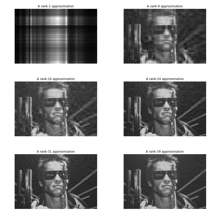
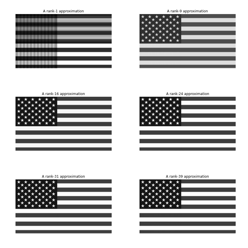
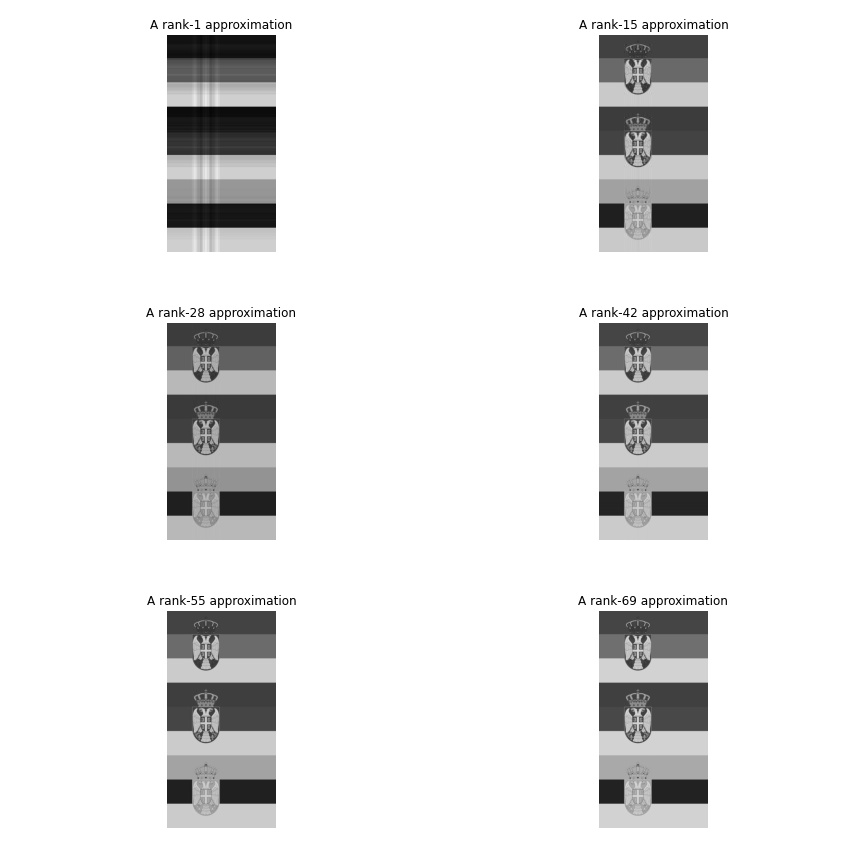
Until now we have reconstructed images in grayscale. In the end, we are going to recreate one more image, this time in RGB.
# Load image
img = cv2.iimg = cv2.imread('serbia.png', 1)
plt.imshow(cv2.cvtColor(img, cv2.COLOR_BGR2RGB))
plt.axis('off')
(b, g, r) = cv2.split(img)
img_s = np.vstack([b, g, r])
plt.imshow(img_s, cmap = 'gray')
plt.axis('off')
# we decompose the image
U, S, VT = np.linalg.svd(img_s)
S = np.diag(S)
draw_svd(img_s, U, S, VT, 'gray')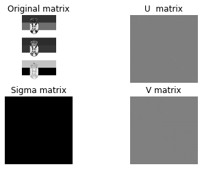
# Rank-r approximation
r_rec = []
g_rec = []
b_rec = []

for r in range(1, 70):
  print(r)
  img_r = np.matmul(U[:,:r] , S[:r,:r])
  img_r = np.matmul (img_r , VT[:r,:])

  r_rec.append(img_r[:800, :])
  g_rec.append(img_r[800:1600, :])
  b_rec.append(img_r[1600:2400, :])

  plt.title(f"A rank-{r} approximation")
  plt.imshow(img_r, cmap='gray')
  filename = "image_" + str(r).zfill(3) + ".jpg"
  plt.axis('off')
  plt.savefig(filename)
When we combine the images, we get a GIF like this:
for i in range(39):
  print(i)
  img_new = cv2.merge([r_rec[i], g_rec[i], b_rec[i]])
  plt.title("first terms of a rank-"+ str(i) +" approximation")
  plt.imshow(cv2.cvtColor(img_new.astype(np.uint8), cv2.COLOR_BGR2RGB))
  filename = "original_image_"+ str(i)+".jpg"
  plt.axis('off')
  plt.savefig(filename)
png_dir = '../content'
images = []
for file_name in sorted(os.listdir(png_dir)):
if file_name.startswith('original_image_'):
file_path = os.path.join(png_dir, file_name)
images.append(imageio.imread(file_path))
imageio.mimsave('../content/movie1.gif', images, fps = 1)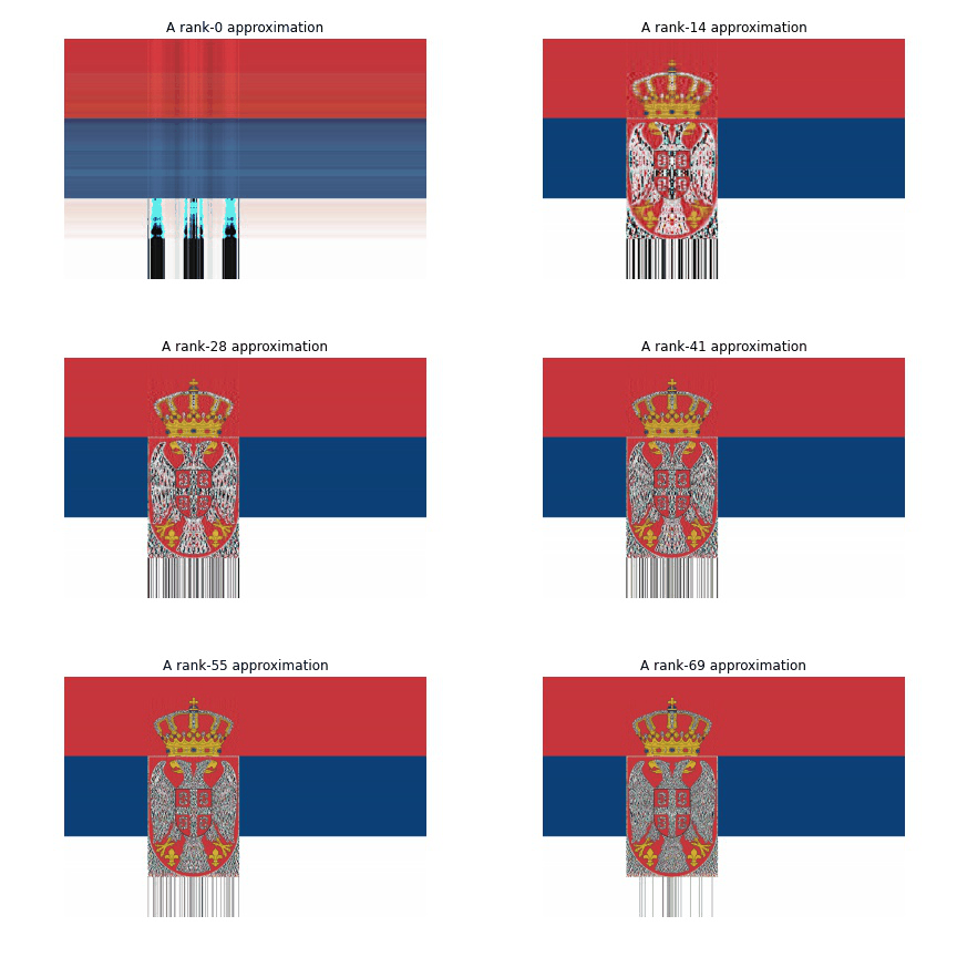
Summary
In this post, we provided a detailed explanation of the very important algorithm in Linear Algebra. We explained that SVD is a matrix decomposition process that will create a set of new matrices. When we multiply back these matrices, we will be able to reconstruct our original matrix. Also, we explained how to implement the SVD algorithm in the Python code. Moreover, we saw how SVD can be used for finding data structures as well as can be applied for the compression.