#007 OpenCV projects – Image segmentation with Watershed algorithm

Highlights: In this post, we are going to cover one of the most important techniques in image processing. We will discuss how to segment an image into different regions. This is an important step in many computer vision applications because it isolates the desired region from the image for further processing tasks. Initially, we will give an overview of the segmentation and start with one of the most common region-based segmentation methods – the Watershed algorithm.

Tutorial overview:

1. What is image segmentation?
2. Different techniques for image segmentation
3. Image segmentation with a Watershed algorithm
4. Image segmentation with the Watershed algorithm in Python
5. Marker-based Watershed segmentation with the K means algorithm

1. What is image segmentation?

Image segmentation is the process of partitioning a digital image into multiple segments by grouping together pixel regions with some predefined characteristics. Each of the pixels in a region is similar with respect to some property, such as color, intensity, location, or texture. It is one of the most important image processing tools because it helps us to extract the objects from the image for further analysis. Moreover, the accuracy of the segmentation step determines success and failure in further image analysis.

You probably wonder what is the use of partitioning an image into several parts. Let’s better understand image segmentation using the following example.

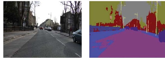
On the left side, we can see the image of the road and on the right, we can see segmented image into several areas – road area, sidewalk area, pedestrian area, tree area, building area, and sky area. Each region is painted in different colors. From this example, it is easy to understand why image segmentation is much more accurate than simple object detection. By using the object detection, we are detecting a set of bounding boxes that correspones to each object in the image. However, to obtain any information about the shape of that object we need a different approach. As you can see, the image segmentation creates a pixel-wise mask for each object of interest in the image that provides us more information about that object.

Why do we need image segmentation?

There are numerous applications of image segmentation in real case scenarios. Let’ see some of them.

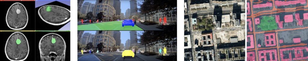
• Medical image processing – analysis of the medical images (MRI, X-ray) for the purpose of detecting diseases as quickly as possible.
• Self Driving Cars – assistance to autonomous cars to better understand their surrounding by recognizing the road cars and pedestrians, with high accuracy
• Satellite images – locating objects in satellite images and significantly reducing the time required to prepare an accurate satellite map

2. Different techniques for image segmentation

There are various Image Segmentation techniques that we can use to distinguish between objects of interest from the image. The segmentation algorithms are categorized according to two basic properties of intensity values: discontinuity and similarity.

• The discontinuity approach splits an image according to sudden changes in intensities (edges).
• The similarity approach splits an image based on similar regions according to predefined criteria

3. Image segmentation with a Watershed algorithm

One of the most popular methods for image segmentation is called the Watershed algorithm. It is often used when we are dealing with one of the most difficult operations in image processing – separating similar objects in the image that are touching each other. To understand the “philosophy” behind the watershed algorithm we need to think of a grayscale image as a topographic surface. In such an image high-intensity pixel values represent peaks (white areas), whereas low-intensity values represent valleys – local minima (black areas).

Now, imagine that we start filling every isolated valley with water. What will happen? Well, the rising water from different valleys will start to merge. To avoid that, we need to build barriers in the locations where the water would merge. These barriers we call watershed lines and they are used to determine segment boundaries. Then, we continue filling water and building watershed until the water level reaches the height of the highest peak. At the end of the process, only watershed lines will be visible and that will be the final segmentation result. So, we can conclude that the goal of this algorithm is to identify watershed lines.

In essence, we partition the image into two different sets: the dark areas are called catchment basins – the group of connected pixels with the same local minimum. Lines that divide one catchment area from another are called watershed lines. The watershed segmentation in 2D is represented in the following image.

As you can see when we rise the yellow threshold eventually segment 1 and segment 2 will be merged, Therefore, we need to put the first watershed line. Afterward, segment 2 and segment 3 will be merged so we need to add another watershed line.

The key problem that we need to solve is how to create an image to which we will apply the Watershed algorithm. Our first choice may be to apply the Gradient magnitude method on the image. However, this method in practice produces an over-segmented result due to noise or some other irregularities in the image. We can obtain more accurate results if we use the distance transform method. We will cover this method leather in the post in more detail.

In addition, we can apply much more advanced processing if we use the marker-based method. These markers will allow us to redefine the regions in advance and thus get much better results.

Now, let’s see how we can apply the Watershed algorithm using Python with OpenCV.

4. Image segmentation with the Watershed algorithm in Python

First, let’s import the necessary libraries.

import cv2
import numpy as np
import skimage
from skimage.feature import peak_local_max
from scipy import ndimage as ndi

import matplotlib.pyplot as plt
from google.colab.patches import cv2_imshowCode language: JavaScript (javascript)

To better understand how the Watershed algorithm works, let’s create a simple binary image of two partially overlapping circles.

img = np.zeros((256, 256),dtype="uint8")
cv2.circle(img, (70,70), 50, (255,255,255), (-1))
cv2.circle(img, (140,140), 70, (255,255,255), (-1))Code language: JavaScript (javascript)

Calculating a distance transform

Now we need to somehow separate these two touching objects and create a border between them. The idea is to create a border as far as possible from the centers of the overlapping objects. For this, we will use the method that works very well on rounded objects and it is called a distance transform. It is an operator that generally takes binary images as inputs and pixel intensities of the points inside the foreground regions are replaced by their distance to the nearest pixel with zero intensity (background pixel).

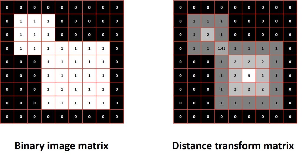
As you can see in the image above every pixel with a value of zero (black pixel) also has a distance transform value of 0, as it is the closest zero-valued pixel to itself. On the other hand, the distance transform of the pixels with the value of 1 is given by the following formula:

$$ d(p_{1}, p_{2})=\sqrt{\left(x_{1}-x_{2}\right)^{2}+\left(y_{1}-y_{2}\right)^{2}} $$

Here the distance \(d(p_{1}, p_{2}) \) represents the Eucledian distance between a point \(p_{1} \) with coordinates \((x_{1},y_{1}) \) and a point \(p_{2} \) with coordinates \((x_{2},y_{2}) \).

So, from this example, we can conclude that pixels closest to the center of our object will have a larger distance transform value.

To apply distance transform in OpenCV we can use the function cv2.distanceTransform(). This method consists of the following parameters:

• src − input image.
• dst − output image.
• distanceType − A variable that represents the type of distance transformation
• maskSize − A variable representing the mask size (usually it is set to a value 3)

For the parameter distanceType we can choose several different types of a distance transform. In our code, we are using a simple Euclidean distance. In the following example, you can see some other types of distance transform.

• DIST_USER – User-defined distance
• DIST_L1 – \(distance = |x_{1}-x_{2}|+| y_{1}-y_{2} \mid \)
• DIST_L2  – the simple Euclidean distance
• DIST_C  – \(distance = max(|x_{1}-x_{2}|,| y_{1}-y_{2} \mid) \)

dist_transform = cv2.distanceTransform(img, cv2.DIST_L2,3)
cv2_imshow(dist_transform)

Finding local maxima points

The next step is to find the coordinates of the peaks (local maxima) of the white areas in the image. For that, we will use the function peak_local_max()from the Scikit-image library. We will apply this function to our distance_transform image and the output will give us the markers which will be used in the watershed function.

local_max_location = peak_local_max(dist_transform, min_distance=1, indices=True)
local_max_boolean = peak_local_max(dist_transform, min_distance=1, indices=False)

print(local_max_boolean)Code language: PHP (php)

[[False False False ... False False False]
 [False False False ... False False False]
 [False False False ... False False False]
 ...
 [False False False ... False False False]
 [False False False ... False False False]
 [False False False ... False False False]]

The optional parameter indices determines the type of the output array. By default, the parameter is set to True, when the output will be an array representing peak coordinates. If it is set to False like in our case, the output will be a boolean array where peaks are represented as True elements.

Note that this function consists of another optional parameter min_distance that determines the minimum number of pixels that separate two peaks in a region. To find the maximum number of peaks we use min_distance=1. To better understand this parameter take a look at the following example.

img1 = np.zeros((7, 7))
img1[2, 2] = 4
img1[2, 4] = 7
print(img1)Code language: PHP (php)

[[0. 0. 0. 0. 0. 0. 0.]
 [0. 0. 0. 0. 0. 0. 0.]
 [0. 0. 4. 0. 7. 0. 0.]
 [0. 0. 0. 0. 0. 0. 0.]
 [0. 0. 0. 0. 0. 0. 0.]
 [0. 0. 0. 0. 0. 0. 0.]
 [0. 0. 0. 0. 0. 0. 0.]]

peak_local_max(img1, min_distance=1)

array([[2, 4],
       [2, 2]]

peak_local_max(img1, min_distance=2)

array([[2, 4]])

As you can see we have created \(7\times7 \) pixels image of all zeros. In addition, we set just two non-zero points at coordinates (2, 2) and (2, 4) with values 4 and 7. Then, we have applied the function peak_local_max() with parameter min_distance. In the first example min_distance=1 the function returns coordinates of both local maximum points. In the second example min_distance=2 the function returns coordinates of the highest peak in the region which is 7 in our case.

Labeling the markers

Now, let’s continue with our code. The next step is to label markers for the watershed function. For that, we will use the function ndi.label()from the SciPy library. This function consists of one parameter input which is an array-like object to be labeled. Any non-zero values in this parameter are considered as features and zero values are considered to be the background. In our code, we will use the coordinates of the calculated local maximum. Then, the function ndi.label()will randomly label all local maximums with different positive values starting from 1. So, in case we have 10 objects in the image each of them will be labeled with a value from 1 to 10.

markers, _ = ndi.label(local_max_boolean)

The final step is to apply the skimage.segmentation.watershed()function from the Scikit-image library. As parameters, we need to pass our inverted distance transform image and the markers that we calculated in the previous line of code. Since the watershed algorithm assumes our markers represent local minima we need to invert our distance transform image. In that way, light pixels will represent high elevations, while dark pixels will represent the low elevations for the watershed transform.

segmented = skimage.segmentation.watershed(255-dist_transform, markers, mask=img)

With the following code snippet, we will plot our original image, inverted distance transform image, and the output image.

fig, axes = plt.subplots(ncols=3, figsize=(9, 3), sharex=True, sharey=True)
ax = axes.ravel()

ax[0].imshow(img, cmap=plt.cm.gray)
ax[0].set_title('Input image')
ax[1].imshow(-dist_transform, cmap=plt.cm.gray)
ax[1].set_title('Distance transform')
ax[2].imshow(segmented, cmap=plt.cm.nipy_spectral)
ax[2].set_title('Separated objects')

for a in ax:
    a.set_axis_off()

fig.tight_layout()
plt.show()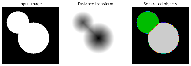Code language: PHP (php)

As you can see we have detected the watershed line right in the middle of the two overlapping circles. It is important to remember that the function skimage.segmentation.watershed()will automatically paint objects that we want to segment with different colors whereas the background area will have a value of zero.

5. Marker-based Watershed segmentation with the K means algorithm

Now, let’s apply the Watershed algorithm on another more complex image with multiple overlapping oranges.

img = cv2.imread('Oranges.jpg')
cv2_imshow(img)Code language: JavaScript (javascript)

The first step is to convert the image into grayscale and to apply the threshold function the cv2.threshold()to separate pixels into the foreground, and the background areas.

gray = cv2.cvtColor(img, cv2.COLOR_BGR2GRAY)
ret, thresh_img = cv2.threshold(gray, 120, 255, cv2.THRESH_BINARY)
cv2_imshow(thresh_img)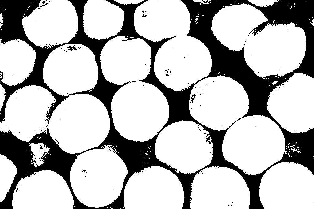

To remove some noise from an image, we use the morphological function morphologyEx(). This function can be used for several morphological operations, so we will need to add a parameter to specify which one we want to use. Since our goal here is to remove small black holes inside the object we will use opening operation (erosion followed by dilation). In this case, we will use four iterations iterations=4 (to suppress larger noise areas we will use more iterations).

# Noise removal
kernel = np.ones((3),np.uint8)
opening_img = cv2.morphologyEx(thresh,cv2.MORPH_OPEN, kernel, iterations = 9)

cv2_imshow(opening_img)Code language: PHP (php)

As you can see we have achieved our goal and removed small black dots from white areas. However, notice that the shapes of some oranges are a little distorted. Since we don’t want to affect the overall shapes of the objects we will apply closing operation (dilation followed by erosion).

# Noise removal
closing_img = cv2.morphologyEx(thresh,cv2.MORPH_CLOSE, kernel, iterations = 4)

cv2_imshow(closing_img)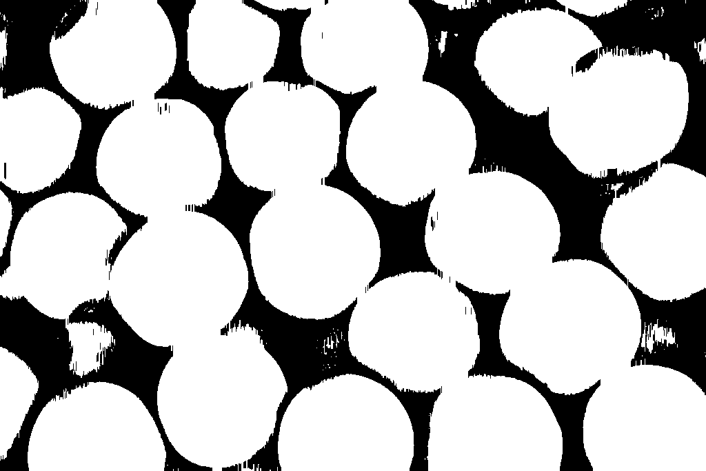Code language: PHP (php)

Next, by applying a distance transform on the opening image we will create a border between touching objects. We will also invert the opening image because the Watershed algorithm assumes that markers represent a local minimum.

dist_transform = cv2.distanceTransform(255 - closing_img, cv2.DIST_L2, 3)
cv2_imshow(dist_transform)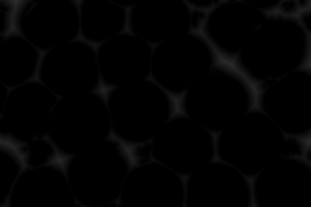

Now, we need to extract the coordinates of the local maximum using the function peak_local_max().

local_max_location = peak_local_max(dist_transform, min_distance=1, indices=True)Code language: PHP (php)

Labeling the markers with K-means algorithm

The next step is to label our local maximums. However, this will not be such a straightforward task like in the previous example when we segmented two connected circles. Now, we are processing a much more complicated image with a large number of local maximums. In some locations, these points will be clustered (scattered) and it will be impossible to label them. For example, if we now apply the function ndi.label()at multiple locations we will have local maximums labeled with the same number. So, how can we solve this problem?

The solution is actually quite easy. We can easily solve our problem if we assign local maximum points to different clusters based on the distance between them. For that, we can use the K-means clustering algorithm.

from sklearn.cluster import KMeans
kmeans = KMeans(n_clusters=30)
kmeans.fit(local_max_location)
local_max_location = kmeans.cluster_centers_.copy()Code language: JavaScript (javascript)

First, we will import the K Means algorithm from the sklearn library. Next, we will set the number of clusters to 30 and calculate K means clustering with a method kmeans.fit(). The parameter of this function will be an array of all coordinates of the local maximum points. Then, we will compute the centers of each cluster and assign them to the local maximum location. In that way, we will have only 30 local maximums.

Now let’s visualize the locations of all 30 local maximum points. Note that K -Means will return a float data type so we need to convert all local maximum locations to an integer.

# Kmeans is returning a float data type so we need to convert it to an int. 
local_max_location = local_max_location.astype(int)Code language: PHP (php)

In the following block, we will create a copy of the distance transform image, and then we will loop over all coordinates in the local maximum array. Then, we will draw a circle in each location in dist_transform_copy image.

local_max_location.shape
dist_transform_copy = dist_transform.copy()
for i in range(local_max_location.shape[0]):
  cv2.circle( dist_transform_copy, (local_max_location[i][1],local_max_location[i][0]  ), 5, 255 )

cv2_imshow(dist_transform_copy)

The next step is to label our markers for the watershed function. With the following code, we will create the image called markers with the same dimensions as the distance transform image. As we know that the number of local maximum points is equal to the number of the clusters, we will arbitrarily assign a number from 1 to 30 to each center of the cluster. These numbers will be our labels.

markers = np.zeros_like(dist_transform)
labels = np.arange(kmeans.n_clusters)
markers[local_max_location[:,0],local_max_location[:,1]   ] = labels + 1

# Convert all local markers to an integer. This because cluster centers will be float numbers. 
markers = markers.astype(int)Code language: PHP (php)

markers_copy = markers.copy()
index_non_zero_markers = np.argwhere(markers != 0)

markers_copy = markers_copy.astype(np.uint8)

index_non_zero_markers
font = cv2.FONT_HERSHEY_SIMPLEX
for i in range(index_non_zero_markers.shape[0]):
  string_text = str(markers[index_non_zero_markers[i][0] ,index_non_zero_markers[i][1]    ])
  cv2.putText( markers_copy, string_text, (index_non_zero_markers[i][1], index_non_zero_markers[i][0]), font, 1, 255)

cv2_imshow(markers_copy)

Now we know that our labels are located in areas where watershed lines suppose to be (non-zero pixels). Finlay, we can apply segmentation. This time we will use the OpenCV version of the watershed algorithm. Do note that before applying cv2.wathershed() function we need to convert out markers image into integer type np.int32.

markers = markers.astype(np.int32)
segmented = cv2.watershed(img, markers)
cv2_imshow(segmented)
print(segmented)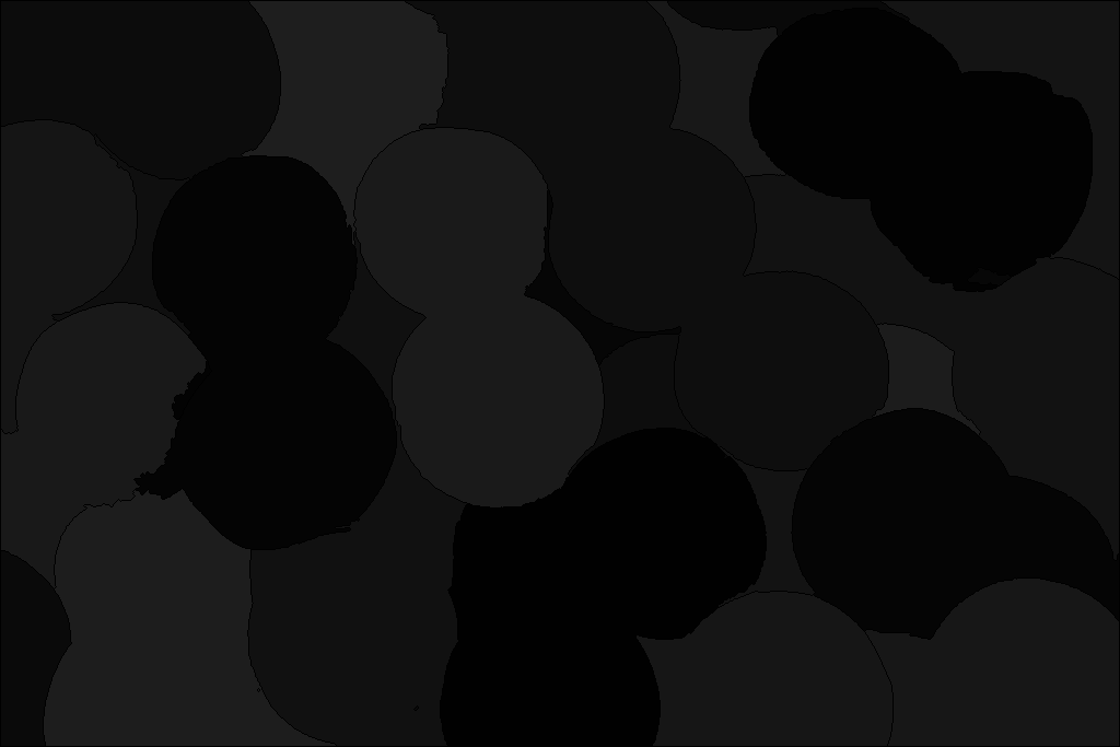Code language: PHP (php)

[[-1 -1 -1 ... -1 -1 -1] 
 [-1 12 12 ... 20 20 -1] 
 [-1 12 12 ... 20 20 -1] 
 ... 
 [-1 10 10 ... 23 23 -1] 
 [-1 10 10 ... 23 23 -1] 
 [-1 -1 -1 ... -1 -1 -1]]

So, we can see how our segmented image looks like. The cv2.wathershed()will update our markers according to the labels we gave. Each pixel will get a different intensity value depending on the nearest label (label 1 will get the lowest value and label 30 will get the highest value). The boundaries of objects will have a value of -1.

For the visualization purpose, we can apply one cool technique. We can display the label matrix as a color image by using built-in colormaps in Matplotlib. Parameter cmap="jet" returns the jet colormap as a three-column array with the same number of rows as the colormap for the input image. Each row in the array contains the red, green, and blue intensities for a specific color. Using this parameter we will map black pixels to blue and white pixels to red color. The gray intensities in between black and white will be mapped to colors between blue and red in the following color shame.

dpi = plt.rcParams['figure.dpi']
figsize = img.shape[1] / float(dpi), img.shape[0] / float(dpi)

plt.figure(figsize=figsize)
plt.imshow(segmented, cmap="jet")
filename = "markers.jpg"
plt.axis('off')
plt.savefig(filename, bbox_inches = 'tight', pad_inches = 0)Code language: JavaScript (javascript)

The next step is to overlay our original image with the image that we just created. To do that we need to create copies of the original image and the overlay image.

from PIL import Image

overlay = cv2.imread("markers.jpg")
overlay = np.asarray(overlay)Code language: JavaScript (javascript)

img_copy = img.copy()
overlay_copy = overlay.copy()

Now, we will resize the overlay copy to fit the shape of the original image. Finally, we will use the function cv2.addWeighted to blend these two images together.

overlay_copy = cv2.resize(overlay_copy, (img_copy.shape[1], img_copy.shape[0]))
final_img = cv2.addWeighted(overlay_copy, 0.5, img_copy, 0.5,	0)

cv2_imshow(final_img)

Now, it is time for the final step. We just need to change the color of the boundary region and pass it to the original image. In that way, we will obtain our watershed lines.

img_c = img.copy() 
img_c[segmented == -1] = [255, 0, 0]
cv2_imshow(img_c)

As you can see the result is quite satisfying but not perfect. Remember that segmenting an image with touching and overlapping object is a very difficult task. Usually, you need to experiment to get the best results for your purpose. However, in this post, we covered all steps for the segmentation with the Watershed algorithm. You can see these steps in the following image.

Summary

In this post, we briefly covered different image segmentation techniques. Moreover, we have explained how the watershed algorithm works. Furthermore, we learned how to segment an image into different regions in order to extracts the objects of interest for further analysis. Finally, we demonstrated how to use one of the well-known image segmentation methods called the Watershed algorithm. In the next post, we will explain how to apply thresholding for image segmentation.

References:

[1] Medical image computing

[2] Pixel-Perfect Perception: How AI Helps Autonomous Vehicles See Outside the Box

[3] Scalable Feature Extraction with Aerial and Satellite Imagery

[4] Image segmentation and mathematical morphology

[5] Marker-Controlled Watershed Segmentation

[6] Watershed segmentation