Highlights: Hello and welcome! In the previous post, we saw how a neural network works in a demand prediction example. Moreover, we learned that the Neural Network architecture is made of individual units called neurons that mimic the biological behavior of the brain. In this post, we are going to take a closer look into the layer of neurons – fundamental building blocks of neural networks. You’ll learn how to construct a layer of neurons and once you have that down, you’d be able to take those building blocks and put them together to form a large neural network. 

Tutorial Overview:

1. Neural network layer
2. Making prediction – Forward propagation
3. Backpropagation
4. How to train a Neural Network in Python

1. Neural network layer

Let’s take a look at how a layer of neurons works. Let’s take a look at the following image.

In this example, we can see a network of three layers. We have four input features in the input layer, then we have the hidden layer of three neurons, and finally, we have the output layer with just one neuron. Let’s take a closer look at the hidden layer and its computations. 

As you can see this hidden layer inputs four numbers and these four numbers are inputs to each of three neurons. Each of these three neurons is just implementing a logistic regression function. 

So, computing an output of a Neural Network is like computing an output in Logistic Regression, but repeating it multiple times. 

The first node in the hidden layer has two parameters, \(w \) and \(b \). 

To denote that this is the first hidden unit, we are going to subscript these parameters as \(w_{1} \) and  \(b_{1} \). This unit will output some activation value \(a_{1} \). Here, we can also see the \(z \) value where \(g(z) \) is the familiar logistic function. Now, we will calculate the output value for each of the three units using the same equations.

After computing the outputs of the hidden layer we will get the vector of three activation values. Then this vector becomes the input to the next layer. In this example, this is the output layer of this neural network. 

Because the output layer has just a single neuron, all it does is it computes \(a_{2} \). This output is just a scalar, is a single number rather than a vector of numbers. Once the neural network has computed \(a_{2} \), there’s one final optional step that you can choose to implement or not, and that is a binary prediction. You can take the number that we computed, and set the threshold at 0.5. If the number is greater than 0.5, you can predict that prediction \(\hat{y}=1 \). On the other hand, if it is less than 0.5, then you can predict that \(\hat{y}=o \). 

So that’s how a neural network works. Every layer inputs a vector of numbers and applies a bunch of logistic regression units to it. After that, it computes another vector of numbers that then gets passed from layer to layer until we get to the final output which is the prediction of the neural network. Then we can set the threshold at 0.5 to come up with the final prediction. 

So, you learned how to compute the activations of any layer given the activations of the previous layer. Now, let’s see how we can get a neural network to make predictions. 

2. Making predictions – Forward propagation

Let’s take what we’ve learned and put it together into an algorithm to let your neural network make inferences or make predictions. This will be an algorithm called forward propagation. 

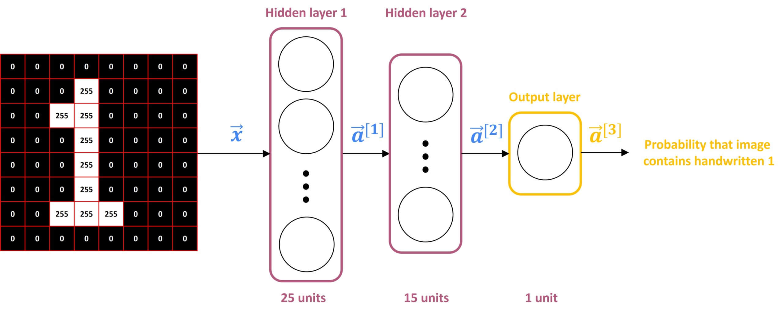
Here we are going to use an example of handwritten digit recognition. For simplicity, we are just going to distinguish between the handwritten digits –  zero and one. So it’s just a binary classification problem where we’re going to input an image and classify this image into two classes – the digit zero and the digit one. 

For this example, we will use a \(8\times8 \) pixels image. As you can see in the following illustration, this image is a matrix of 64-pixel intensity values where 255 denotes a bright white pixel and zero would denote a black pixel. Given these 64 input features, we’re going to use the neural network with two hidden layers, where the first hidden layer has 25 neurons and the second hidden layer has 15 neurons. Finally, the output layer consists of only a single neuron. So let’s step through the sequence of computations that we need to make to go from the input image \(\vec{x} \), to the predicted probability \(a_{3} \).

The first computation goes from \(\vec{x} \) to  \(a_{1} \), and it carries out the following  computation:

$$ \vec{a}^{[1]} = \begin{bmatrix}g(\vec{w}_{1}^{[1]} \vec{x}  + b_{1}^{[1]}) \\\vdots \\g(\vec{w}_{25}^{[1]} \vec{x}  + b_{25}^{[1]})\end{bmatrix} $$

Here, a superscript square bracket denotes the layer. Also, notice that this matrix has 25rows because this hidden layer has 25 units. 

The next step is to compute \(a_{2} \). Looking at the second hidden layer, it then carries out this computation where \(a_{2} \) is a function of \(a_{1} \) and it’s computed using the following equation: 

$$ \vec{a}^{[2]} = \begin{bmatrix}g(\vec{w}_{1}^{[2]} \vec{a^{[1]}}  + b_{1}^{[2]}) \\\vdots \\g(\vec{w}_{15}^{[2]} \vec{a^{[1]}}  + b_{15}^{[2]})\end{bmatrix} $$

Notice that the second layer has 15 neurons, which is why parameters 1 through 15 

The final step is then to compute \(a_{3} \). For that, we will use a very similar computation. The only difference is that this third layer has just one unit. That is why there’s just one output here. 

$$ \vec{a}^{[3]} = g(\vec{w}_{1}^{[3]} \vec{a^{[2]}}  + b_{1}^{[3]}) $$

So \(a_{3} \) is just a scalar. We can now take this scalar and threshold it at 0.5 to come up with a binary classification label.

This algorithm is also called forward propagation because you’re propagating the activations of the neurons. So you’re making these computations in the forward direction from left to right. And this is in contrast to a different algorithm called backward propagation or backpropagation, which is to compute the gradients. 

3. Backpropagation

The backpropagation algorithm aims to minimize the cost function by adjusting the network’s weights and biases.  It is a technique used in training neural networks to update the weights and biases by calculating the gradient so that the accuracy of the neural network can be improved iteratively.

In the post Logistic regression, we already explained which equations we need to use to update [aramethers \(w \) and \(b \). The following backpropagation graph describes which calculations we need to make when we want to calculate various derivatives and update the parameters. We can see that it is similar to the Logistic Regression only now we need to calculate derivatives for each layer of the neural network.

So first,  we calculate derivatives of the \(a \), and \(z \) for the last layer. These calculations allow us to calculate \(dw \) and \(db \). Then, as we go deeper into the backpropagation step, we calculate. 

.Now, let’s take a look at how we can implement this knowledge in Python. 

4. How to train a Neural Network in Python?

First, let’s import the necessary libraries that we will use in the Python code.

import numpy as np
import matplotlib.pyplot as plt
from sklearn.datasets import make_circles
from sklearn.datasets import make_moons
import seaborn as sns
sns.set()Code language: JavaScript (javascript)

Here, datasets are linearly non-separable. We have two classes: class 0 and class 1. In the training set, we have 2000 examples (1000 from class 0 and 1000 from class 1) and in the test set, we have 1000 examples (500 from each class).

X,y = make_circles(n_samples = 3000, noise = 0.08, factor=0.3)
#X,y = make_moons(n_samples = 3000, noise = 0.08)
X0 = []
X1 = []
for i in range(len(y)):
    if y[i] == 0:
        X0.append(X[i,:])
    else:
        X1.append(X[i,:])
            
X0_np = np.array(X0)
X1_np = np.array(X1)

X0_train = X0_np[:1000,:].T # we want X to be made of examples which are stacked horizontally
X0_test = X0_np[1000:,:].T
X1_train = X1_np[:1000,:].T
X1_test = X1_np[1000:,:].T

X_train = np.hstack([X0_train,X1_train]) # all training examples
y_train=np.zeros((1,2000))
y_train[0, 1000:] = 1
X_test = np.hstack([X0_test,X1_test]) # all test examples
y_test=np.zeros((1,1000))
y_test[0, 500:] = 1

plt.scatter(X0_train[0,:],X0_train[1,:], color = 'b', label = 'class 0 train')
plt.scatter(X1_train[0,:],X1_train[1,:], color = 'r',  label = 'class 1 train')
plt.scatter(X0_test[0,:],X0_test[1,:], color = 'LightBlue', label = 'class 0 test')
plt.scatter(X1_test[0,:],X1_test[1,:], color = 'Orange', label = 'class 1 test')
plt.xlabel('feature1')
plt.ylabel('feature2')
plt.legend()
plt.axis('equal')
plt.show()

# we will plot shapes of training and test set to make sure that they were made by stacking examoles horizontally
# so in every column of these matrices there is one examples
# in two rows there are features (feature1 is ploted on the x-axis, and feature2 is ploted on the y-axis)
print('Shape of X_train set is %i x %i.'%X_train.shape)
print('Shape of X_test set is %i x %i.'%X_test.shape)
# labels for these examples are in y_train and y_test
print('Shape of y_train set is %i x %i.'%y_train.shape)
print('Shape of y_test set is %i x %i.'%y_test.shape)
Code language: PHP (php)

• Shape of X_train set is 2 x 2000
• Shape of X_test set is 2 x 1000
• Shape of y_train set is 1 x 2000
• Shape of y_test set is 1 x 1000.

The next step is to initialize our parameters. To do that we are going to define a function initialize_parameters() that takes as an input the number of features in a single example from a dataset. In our case n_x = 2 because we have two features (drown on the x-axis and y-axis). Parameters that we are going to use are W1, W2, b1, and b2. Matrices W1 and W2 are initialized with small random values, and biases are initialized with zeros. The output of this function is a Python dictionary that contains values of all these parameters.

def initialize_parameters(n_x, n_h, n_y):
    
    np.random.seed(2) 
    
    W1 = np.random.randn(n_h, n_x) * 0.01
    b1 = np.zeros(shape=(n_h, 1))
    W2 = np.random.randn(n_y, n_h) * 0.01
    b2 = np.zeros(shape=(n_y, 1))
    
    assert (W1.shape == (n_h, n_x))
    assert (b1.shape == (n_h, 1))
    assert (W2.shape == (n_y, n_h))
    assert (b2.shape == (n_y, 1))
    
    parameters = {"W1": W1,
                  "b1": b1,
                  "W2": W2,
                  "b2": b2}
    
    return parametersCode language: JavaScript (javascript)

Now, let’s define the activation functions that we are going to use. First, we will use one familiar function which is the sigmoid function in the output layer. Also, we will use the tanh function in the hidden layer. Another common function that is used in the hidden layer is called the ReLU activation function. In the next post, we are going to dive deeper into the different types of activation functions.

def relu(x):
    return x*(x>0)
def sigmoid(x):
    return 1/(1+np.exp(-x))
def tanh(x):
    return (np.exp(x)-np.exp(-x))/(np.exp(x)+np.exp(-x))Code language: JavaScript (javascript)

The next step is to apply forward propagation. For that, we will define the function forward_pass() that will make calculations for the forward pass through the neural network. It takes the data X and parameters as arguments and outputs the matrix of predictions A2, and dictionary cache. This dictionary contains cached values which we will use in backward propagation calculations.

def forward_pass(X, parameters):
    
    # to make forward pass calculations we need W1 and W2 so we will extract them from dictionary parameters
    W1 = parameters['W1']
    W2 = parameters['W2']
    b1 = parameters['b1']
    b2 = parameters['b2']

    
    # first layer calculations - hidden layer calculations
    Z1 = np.dot(W1, X) + b1
    A1 = tanh(Z1)  # activation in the first layer is tanh
    
    # output layer calculations
    Z2 = np.dot(W2, A1) + b2
    A2 = sigmoid(Z2)# A2 are predictions, y_hat
    
    # cache values for backpropagation calculations
    cache = {'Z1':Z1,
             'A1':A1,
             'Z2':Z2,
             'A2':A2
            }
    
    return A2, cacheCode language: PHP (php)

Now we can define the function backward_pass() which will take parameters, cached values from the forward propagation step, and dataset X with labels Y.

def backward_pass(parameters, cache, X, Y):
    
    # unpack paramaeters and cache to get values for backpropagation calculations
    W1 = parameters['W1']
    W2 = parameters['W2']
    
    Z1 = cache['Z1']
    A1 = cache['A1']
    Z2 = cache['Z2']
    A2 = cache['A2']
    
    m = X.shape[1] # number of examples in a training set
    
    dZ2= A2 - Y
    dW2 = (1 / m) * np.dot(dZ2, A1.T)
    db2 = (1 / m) * np.sum(dZ2, axis=1, keepdims=True)   # keepdims - prevents python to output rank 1 array (n,)
    
    dZ1 = np.multiply(np.dot(W2.T, dZ2), 1 - np.power(A1, 2)) # we use tanh activation function
    dW1 = (1 / m) * np.dot(dZ1, X.T)  
    db1 = (1 / m) * np.sum(dZ1, axis=1, keepdims=True)
    
    grads = {"dW1": dW1,
             "db1": db1,
             "dW2": dW2,
             "db2": db2}
    
    return gradsCode language: PHP (php)

To update parameters after each iteration we are going to use the function update_parameters() .

def update_parameters(parameters, learning_rate, grads):
    
    W1 = parameters['W1']
    b1 = parameters['b1']
    W2 = parameters['W2']
    b2 = parameters['b2']
    
    dW1 = grads['dW1']
    db1 = grads['db1']
    dW2 = grads['dW2']
    db2 = grads['db2']
    
    W1 = W1 - learning_rate * dW1
    b1 = b1 - learning_rate * db1
    W2 = W2 - learning_rate * dW2
    b2 = b2 - learning_rate * db2
    
    # updated parameters
    parameters = {"W1": W1,
                  "b1": b1,
                  "W2": W2,
                  "b2": b2}
    
    return parametersCode language: PHP (php)

The following function NN_model() calculates optimal values for parameters. Here we will iterate through a number of iterations, apply a forward pass, calculate the cost, apply a backward pass, and finally update the parameters.

def NN_model(X,Y,n_h, num_iterations, learning_rate):
    
    n_x = X.shape[0] # size of an input layer = number of features 
    n_y = Y.shape[0] # size of an output layer
    parameters = initialize_parameters(n_x, n_h, n_y)
    
    #unpack parameters
    W1 = parameters["W1"]
    b1 = parameters["b1"]
    W2 = parameters["W2"]
    b2 = parameters["b2"]
    
    for i in range(num_iterations):
        A2, cache = forward_pass(X, parameters)
        cost  = cost_calculation(A2, Y)
        grads = backward_pass(parameters, cache, X, Y)
        parameters = update_parameters(parameters, learning_rate, grads)
        
    return parametersCode language: PHP (php)

To make predictions, we have defined the function predict() which takes learned parameters and applies them to calculate predictions.

def predict(parameters, X):
    
    A2, cache = forward_pass(X, parameters)
    predictions = np.round(A2)
    
    return predictionsCode language: JavaScript (javascript)

Now let’s use the function NN_model() to learn parameters. For the process of learning, we will use the training set, and labels for the training set. Also, we will use a shallow neural network with 4 units in the hidden layer. Furthermore, we will define 20 000 iterations and set the learning rate to be equal to 0.1.

num_iterations = 20000
learning_rate = 0.1
n_h = 4
parameters_final = NN_model(X_train,y_train,n_h, num_iterations, learning_rate)

Now, we will make predictions on our test and training set, and we will print the accuracy.

Y_predictions_test = predict(parameters_final, X_test)
Y_predictions_train = predict(parameters_final, X_train)

print("train accuracy: {} %".format(100 - np.mean(np.abs(Y_predictions_train - y_train)) * 100))
print("test accuracy: {} %".format(100 - np.mean(np.abs(Y_predictions_test - y_test)) * 100))Code language: CSS (css)

train accuracy: 99.95 %

test accuracy: 99.9 %

Wow! As you can see we got accuracy close to 100 %. That is an amazing result. However, let’s visualize our data. To do that we will define functions for various plots we have to make.

def plot_grid(parameters_final, X_set):
    x_min, x_max = X_set[0,:].min(), X_set[0,:].max()
    y_min, y_max = X_set[1,:].min(), X_set[1,:].max()

    
    xx, yy = np.meshgrid(np.linspace(x_min, x_max,100),np.linspace(y_min, y_max,100))
    
    G = np.c_[xx.ravel(), yy.ravel()]
    D = G.T
    
    predictions = predict(parameters_final, D)
    predictions = predictions.reshape(10000,)

    #plt.contourf(np.c_[xx.ravel(), yy.ravel()][0], np.c_[xx.ravel(), yy.ravel()][1], D, cmap=plt.cm.Spectral)
    color = {'0':'gray',
             '1':'yellow'}
    predictions_colors = [color[str(int(predictions[i]))] for i in range(len(predictions))]
    
    plt.scatter(D[0,:],D[1,:], c=predictions_colors)Code language: PHP (php)

def plot_classified(X_set,Y_prediction,c_class0, c_class1, title_str, feature_1_str=''):
    
    # c_class0 is a string, a color for class 0; c_class1 is a string, a color for class 1
    
    colors_d = {'0' : c_class0,
                '1' : c_class1}
    
    colors = [colors_d[str(int(Y_prediction[0,i]))] for i in range(Y_prediction.shape[1]) ]
    c = np.array(colors)
    plt.scatter(X_set[0,:], X_set[1,:], color=c)
    plt.xlabel(feature_1_str)
    plt.title(title_str)
    plt.axis('equal')Code language: PHP (php)

def plot_original_set(X_set, y_label, c_class0, c_class1, title_str):
    
    colors_d = {'0' : c_class0,
                '1' : c_class1}
    
    colors = [colors_d[str(int(y_label[0,i]))] for i in range(y_label.shape[1]) ]
    c = np.array(colors)
    plt.scatter(X_set[0,:], X_set[1,:], color=c)
    plt.xlabel('feature1')
    plt.ylabel('feature2')
    plt.title(title_str)
    plt.axis('equal')Code language: PHP (php)

Now that we defined our functions let’s plot how does algorithm classify the training set.

plt.subplot(1,2,1)
plot_original_set(X_train, y_train, 'Blue', 'Red', 'Training set')
plt.subplot(1,2,2)
plot_grid(parameters_final, X_train)
plot_classified(X_train, Y_predictions_train, 'Blue', 'Red', 'Classified', 'feature1' )
plt.show()Code language: JavaScript (javascript)

Now, let’s take a look at how the algorithm does on the test set.

plt.subplot(1,2,1)
plot_original_set(X_test, y_test, 'LightBlue', 'Orange', 'Test set')
plt.subplot(1,2,2)
plot_grid(parameters_final, X_test)
plot_classified(X_test, Y_predictions_test, 'LightBlue', 'Orange', 'Classified', 'feature1' )
plt.show()Code language: JavaScript (javascript)

As you can see all data points in the test set are accurately classified.

Summary

In this post, you learned how to compute the activations of any layer of the Neural Network given the activations of the previous layer. We learned how to make predictions using forward propagation and how to calculate derivatives and update parameters using backpropagation. Finally, we implemented our knowledge in Python by building a simple neural network from strach. In the next post, we will learn how to use different activation functions as an alternative to the sigmoid activation function.