#004 Machine Learning – Logistic Regression Models

Highlights: Welcome back to our ongoing Machine Learning tutorial series. In the previous post, we learned how to enhance the performance of a Linear Regression model and studied the applications of Multiple Linear Regression.

In today’s tutorial post, we will study and implement a Logistic Regression model, covering basic fundamentals of derivatives, overfitting and binary prediction. And, of course, we’ll use Python to boost our understanding of the concepts we study by writing some code. So, let’s begin!

Tutorial Overview:

1. Understanding Binary Classification Problems
   1. Binary Classification Problem: Example
2. Logistic Regression: An Introduction
   1. Sigmoid Function
3. Cost Function Optimization
   1. 3D Plot of a Non-Convex Gradient Descent
   2. Cross-Entropy Loss Function
4. Calculating Logistic Regression Derivatives
5. Understanding Overfitting
   1. Simplifying The Model
   2. Early Stopping
   3. Adding More Data To The Training-Set
   4. Data Augmentation
   5. Regularisation Techniques
   6. Dropouts
6. Logistic Regression In Python

1. Understanding Binary Classification Problems

In the previous post, we learned how to build a Linear Model using a labelled training dataset in order to make predictions. We analysed the inter-dependence between features like the size of the house, number of bedrooms, number of floors, and price of the house. We learned that these types of data have a linear relationship which means that we can predict the price based on the features.

This type of prediction is called Linear Regression. The goal of Linear Regression is to develop a model that could predict any real value. However, in practice, we often come across a situation when we need to predict a specific output that has only two distinct values as is shown in the following examples.

Consider some questions and think about their possible answers:

• Did you pass your exam?
• Are you vaccinated against COVID-19?
• Did your favourite basketball team win?
• If you drive 100 miles per hour, will you reach point B from point A on time?

As you may notice, in all of these examples, there are only two possible answers – Yes or No.

Basically, we try to distinguish between two classes of outcomes. This type of prediction is called Binary Classification. The goal of Binary Classification is to classify elements of a given set of data into two groups.

Binary Classification Problem: Example

In the following image, we can see an example of a binary classification problem. Here, for instance, our goal is to classify the given image into two classes. Have a look.

• \(x \) represents our input image
• \(y \) denotes the output; it is a label with which we can recognize the image
• \(y \) can only have two values, 1 or 0; if \(y=1 \), there is a cat in an image; else, if \(y=0 \), there is no cat in the image

Therefore, the task of Binary Classification is to learn a classifier that can take an image represented by its feature vector \(x \), and predict whether the corresponding label is 1, i.e., a cat is in an image, or 0, i.e., no cat in the image. In other words, we need an algorithm to output the prediction \(\hat{y} \) which is an estimate of \(y \).

Let’s study further and see what’s the best way to solve such Binary Classification problems.

2. Logistic Regression: An Introduction

One of the most common algorithms that are used to solve Binary Classification problems is called Logistic Regression. It is a Supervised Learning algorithm that we can use when labels are either 0 or 1.

$$ \hat{y}= P\left ( y=1|x \right) \\x\in \mathbb{R}^{n_x}$$

Here, \(\hat{y} \) is the chance of \(y =1 \) given the input features \(x \). Also, \(x \) is an \(n_{x}\) – dimensional vector. The parameters of Logistic Regression are \(w \), which is also an \(n_{x}\) – dimensional vector, together with \(b \) which is a real number.

$$ \mathrm{Parameters}: w \in \mathbb{R}^{n_x}, b \in \mathbb{R}$$

Now, the question arises that given an input \(x \), and the parameters \(w \) and \(b \), how do we generate the output? One thing we could try is to apply the linear function:

$$ \hat{y}=w^{T}x+b $$

However, this is not a very good algorithm for Binary Classification because we want \(\hat{y} \) to be the chance that \(y =1 \). Therefore, \(\hat{y} \) should be in the range between 0 and 1. It is difficult to enforce this because \(\hat{y} \) can be much bigger than 1. It can also be a negative number.

Here, we can conclude that we need a function that will transform our linear function to be within the range of 0 and 1. To do this, we will apply the Sigmoid Function.

Sigmoid Function

In the following image, we can see a set of images. Some of them have a cat and some are non-cat images.

So, instead of fitting a line to the data (as in Linear Regression), Logistic Regression fits an “S” shaped logistic function called the Sigmoid Function.

A Sigmoid Function is a type of activation function that restricts the output to a range between 0 and 1. If you need a more detailed explanation of the Sigmoid Function, you can visit this link.

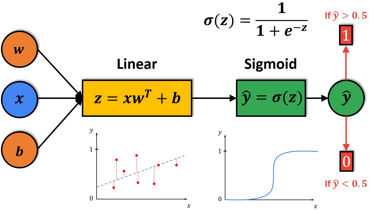
To visualize the Logistic Regression model, let’s take a look at the following image.

As you can see, we will first calculate the output of a linear function \(z \). This output \(z \) will be the input to the Sigmoid Function.

Next, for calculated \(z \) we will produce prediction \(\hat{y} \) which will be determined by the \(z \). Then, if \(z \) is large positive value, the \(\hat{y} \) will be close to 1. On the other hand, if \(z \) is a large negative value, the \(\hat{y} \) will be close to 0. Therefore, the \(\hat{y} \) will always be in the range between 0 to 1.

One simple way to classify the prediction \(\hat{y} \) is to use a threshold value of 0.5. So, if our prediction is greater than 0.5, we assume that \(y \) is 1. Otherwise, we will assume that \(y \) is 0. As the \(\hat{y} \) gets closer to 1, the probability that there is a cat in the image becomes higher. On the other hand, as the \(\hat{y} \) comes closer to 0, the probability that there is a cat in the image also becomes lower.

To calculate the \(\hat{y} \), we will use the following equations. It is a very simple calculation wherein we will just plug in the Sigmoid Function formula into the linear model.

Linear Model:

$$ \hat{y}=w^{T}x+b $$

Sigmoid Function:

$$ \sigma(z)=\frac{1}{1+e^{-z}} $$

Logistic Regression Model:

$$ \hat{y}=\sigma(w^{T}x+b) $$

If \(z \) is a large positive number, then:

$$\sigma (z)=\frac{1}{1+0}\approx 1 $$

If \(z \) is a large negative number, then:

$$ \sigma (z)=\frac{1}{1+\infty }\approx 0 $$

So, when we implement Logistic Regression, our primary goal is to attempt computing the parameters \(w \) and \(b \), such that \(\hat{y} \) becomes a good estimate of the chance of \(y=1 \).

In the following section, we’ll see how we can train our parameters and define a crucial element of our model, i.e., the cost function.

3. Cost Function Optimization

Now, to train the parameters \(w \) and \(b \) of our Logistic Regression model, we need to define a Cost Function.

First, let’s remind ourselves how we compute a cost. If you need a quicker refresher, you can check out our post on Linear regression.

Now, for each data point \(x \), we start computing a series of operations to produce a predicted output. Then, we compare this predicted output to the actual output and calculate a prediction error. This error is what we minimize during the learning process using an optimization strategy.

The way we’re computing that error value is by using a Loss Function. Our ultimate goal is to minimize the Loss Function in order to identify the values of \(w \) and \(b \). For this, we use an algorithm called the Gradient Descent.

In Logistic Regression, we also use the Loss (Error) Function, \(\mathcal{L}\), to measure how well our algorithm is doing. Remember that the Loss Function is applied only to a single training sample, and the commonly used Loss Function is the Squared Error Loss Function, as represented below:

$$ \mathcal{L}(\hat{y},y) = \frac{1}{2}(\hat{y} – y)^{2} $$

In the case of Linear Regression, a loss function is a convex function or a bowl shape. Have a look at the following image to see how the loss function will look for Linear Regression and Logistic Regression.

In Linear Regression, Gradient Descent will take one step at a time until it converges at the global minimum.

Now, you could try to use the same Cost Function for Logistic Regression. But, it turns out that the plot for the Cost Function becomes what’s called a Non-Convex Cost Function. What this means is that in this case, there are lots of local minima.

Interestingly, in Logistic Regression, this Squared Error Cost Function is not a good choice. Instead, there will be a different Cost Function that can make the Cost Function convex again. The Gradient Descent can be guaranteed to converge to the global minimum. 

Now, it is a good moment to see what is the difference between convex and non-convex problems. 

Let’s assume you are standing at some point inside a closed set (like a field surrounded by a fence). Suppose that you can see the entire boundary just by taking a \(360^{\circ} \) turn around yourself. In such a case, the set is convex.

On the other hand, if there is some part of the boundary that you can’t possibly see from where you stand and you have to move to another point to be able to see it, then the set is non-convex.

3D Plot of a Non-Convex Gradient Descent

In terms of a surface, the surface is convex if, loosely speaking, it looks like a ‘cup’ (like a parabola). If you have a ball and you let it roll along the surface, the surface is said to be convex if that ball is guaranteed to always end up at the same point in the end. However, if the surface has ‘bumps’, then, depending on where you drop the ball from, it might get stuck somewhere else. In this case, the surface is non-convex.

Cross-Entropy Loss Function

To be sure that we will get to the global optimum, will use the Cross-Entropy Loss. It measures the performance of a classification model whose output is a probability value between 0 and 1.

In the graph above, we can see that the Cross-Entropy Loss increases as the predicted probability diverge from the actual label. As the predicted probability approaches value 1, log loss slowly decreases. Here, a perfect model would have a log loss of 0.

In Binary Classification, when we have only two classes, Cross-Entropy can be calculated using the following equation:

$$ \mathcal{L}(\hat{y},y)=-(ylog\hat{y}+(1-y)log(1-\hat{y})) $$

It will give us a convex optimization and therefore, it will be much easier to optimize our parameters. 

To understand why this is a good choice, let’s see these two cases:

• If \(y \) = 1,
  • \(\mathcal{L}( \hat{y}, y) = – log \hat{y} \)  \(\Rightarrow \)  \(log \hat{y}\) should be large, so, we want \(\hat{y} \) large (as close as possible to 1 ) 
• If \(y \) = 0,
  • \(\mathcal{L}( \hat{y}, y) = – log (1 – \hat{y}) \) \(\Rightarrow \)  \(log (1 – \hat{y})\) should be large, so, we want \(\hat{y} \) small (as close as possible to 0 ) 

Remember, \(\hat{y}\) is a Sigmoid Function such that it cannot be less than 0 and bigger than 1.

Now, we can define our Cost Function which measures how well our parameters \(w \) and \(b \) are doing on the entire training set. Here, we will use \((i) \) superscript to index different training examples.

$$ J(w, b) = \frac{1}{m}\sum_{i=1}^{m}\mathcal{L}(\hat{y}^{(i)},y^{(i)})=-\frac{1}{m}\sum_{i=1}^{m}\hat{y}^{(i)}log\hat{y^{(i)}}+(1-y^{(i)})log(1-\hat{y}^{(i)}) $$

• Cost Function, \(J\), is defined as the average of the sum of Loss Functions, ( \( \mathcal{L} \) ) of all parameters
• Cost Function is a function of parameters \(w \) and \(b\)

In the following Cost Function diagram, the horizontal axes represent our spatial parameters, \(w \) and \(b \), respectively.

Note, that in practice, \(w \) can be of a much higher dimension, but, for the purpose of plotting, we have illustrated \(w \) and \(b \) as scalars. The Cost Function, \(J(w,b) \), is some surface above these horizontal axes, \(w \) and \(b \). So, the height of the surface represents the value of \(J(w,b) \) at a certain point. Our goal, here, is to minimise the function, \(J \), and to find parameters \(w \) and \(b \) .

4. Calculating Logistic Regression Derivatives

Before we calculate the parameters \(w \) and \(b \), let us take a look at the following computation graph of a Logistic Regression model.

In this example, we only have two features \(x_{1}\) and \(x_{2}\). In order to compute \(z \), we will need to input \(w_{1}\), \(w_{2}\) and \(b \), in addition to the feature values \(x_{1}\) and \(x_{2}\), as shown below:

$$ z = w_{1}x_{1} + w_{2} x_{2} + b $$

Now, we can compute the prediction \(\hat{y} \) as well as the Loss Function, as follows:

$$ \hat{y}  = \sigma(z) $$

$$ \mathcal{L}(\hat{y},y) $$

To reduce our Loss Function (remember, right now, we are talking only about one data sample), we have to update our parameters, \(w \) and \(b \). To do this, we will compute the derivatives.

First, we need to calculate the derivative of loss with respect to \(\hat{y} \), as shown below:

$$ \mathcal{L}(\hat{y},y)=-(ylog\hat{y}+(1-y)log(1-\hat{y})) $$

$$ d\hat{y} = \frac{\mathrm{d} \mathcal{L(\hat{y},y)} }{\mathrm{d} \hat{y}} $$

$$ d\hat{y} = – \frac{y}{\hat{y}} + \frac{1-y}{1-\hat{y}} $$

The next step is to compute the derivative of loss with respect to \(z \).

$$ dz = \frac{\mathrm{d} \mathcal{L(\hat{y},y)} }{\mathrm{d}z} $$

$$ dz = \frac{\mathrm{d} \mathcal{L(\hat{y},y)} }{\mathrm{d} \hat{y}} \frac{\mathrm{d} \hat{y} }{\mathrm{d} z} $$

$$ \frac{\mathrm{d} \mathcal{L(\hat{y},y)} }{\mathrm{d} \hat{y}}= – \frac{y}{\hat{y}} + \frac{1-y}{1-\hat{y}} $$

$$ \frac{\mathrm{d} \hat{y}}{\mathrm{d} z} = a(1 – \hat{y}) $$

$$ dz = \hat{y} – y $$

The final step is to compute the amount of change of our parameters \(w \) and \(b \):

$$ {dw_{1}} = \frac{\mathrm{d} \mathcal{L(\hat{y},y)} }{\mathrm{d} w_{1}} = x_{1} {dz} $$

$$ {dw_{2}} = \frac{\mathrm{d} \mathcal{L(\hat{y},y)} }{\mathrm{d} w_{2}} = x_{2} {dz} $$

$$ {db} = \frac{\mathrm{d} \mathcal{L(\hat{y},y)} }{\mathrm{d} b} = {dz} $$

To conclude, if we want to perform Gradient Descent with respect to this particular data sample only, then, we would need to perform the following updates (for some arbitrary number of iterations):

$$ w_{1} = w_{1} – \alpha{dw_{1}} $$

$$ w_{2} = w_{2} – \alpha{dw_{2}} $$

$$ b = b – \alpha{ db} $$

We have successfully learned about two types of learning algorithms, viz., Linear Regression and Logistic Regression. Each of the learning algorithms perform well for many tasks. However, sometimes, in an application, an algorithm can run into a problem known as Overfitting, which can cause it to perform poorly.

In the next section, we will understand what Overfitting is and how to avoid it.

5. Understanding Overfitting

When building a Neural Network our goal is to develop a model that performs well not just on the training dataset, but also on the new data that it wasn’t trained on.

However, when our model is too complex, sometimes it can start to learn irrelevant information in the dataset. This means that the model memorises the noise that is closely related only to the training dataset.

In such a case, the model is highly inaccurate because the memorised pattern does not reflect the important information present in the data. For such a model, we say that it is overfitted and is unable to generalise well to the new data. It has learned the features of the training set extremely well, but if we give the model any data that slightly deviates from the exact data used during training, it’s unable to generalise and thus, unable to accurately predict the output. 

The best way to tell if your model is overfitted is to use a validation dataset during the training. Then, once you realise that the validation metrics are considerably worse than the training metrics you can be sure that your model is overfitted.

The logical response to prevent Overfitting can either be to stop the training process earlier or to reduce the complexity of the network. However, in both of these cases, an opposite problem called Underfitting can occur. Now, this happens when the model has not been trained for enough time and so, it is unable to determine a meaningful relationship between the input and the output variables.

Based on the model’s performance for both training and testing data, we classify our model into three categories:

• Underfit Model: This type of model can’t learn the problem and performs poorly on both training and testing datasets.
• Overfit Model: This type of model learns the training dataset quite well but does not perform greatly on a testing dataset.
• Optimal Model: This type of model not only learns the training dataset well but also performs well on a testing dataset.

The following image illustrates all of the above three scenarios aptly. Have a look.

Now that we learned what Overfitting is, the question that we need to ask is “how can we avoid this problem?” Well, to avoid Overfitting in the Neural Network, we can apply several techniques. Let’s look at some of them. 

Simplifying The Model

The first method that we can apply, to avoid Overfitting, is to decrease the complexity of the model. To do this, we can simply remove the layers and make the network smaller.

Note that while removing the layers, it is important to adjust the input and output dimensions of the remaining layers in the Neural Network. 

Early Stopping

Another common approach to avoid Overfitting is called Early Stopping. If you choose this method, your goal is very simple. You just need to stop the training process before the model starts learning irrelevant information (noise).

However, we mentioned in the previous chapter that if you apply this method, you can end up with the opposite problem of Underfitting. This is why the main challenge of this approach is to find the right point just before your model starts to overfit. This method is illustrated in the following image.

In the image above, the green curve represents the Training Loss and the red curve represents the Validation Loss. As we can see, after several epochs, Validation Loss has started to increase while the Training Loss is still decreasing. Therefore, we can be sure that the model is Overfitting and we can stop the training exactly at the point where Validation Loss has started to increase.

Adding More Data To The Training Set

Probably the easiest way to eliminate Overfitting is to add more data. More the data we have in the training set, more the model will be able to learn from it. In addition, with more data, we also hope to add more diversity to the training set.

Data Augmentation

Data Augmentation is the most popular technique that is used to increase the amount of data in the training set. To get more data, we just need to make minor alterations to our existing dataset. Even though the changes that we are making are quite subtle, our Neural Network will think these are distinct images.

The benefit of Data Augmentation is that the model is unable to overfit all the samples, and is forced to generalise. The most common Data Augmentation techniques are flipping, translation, rotation, scaling, changing brightness, and adding noise. For a more detailed explanation of this topic, check this link.

Regularisation Techniques

Another popular method that we can use to solve the Overfitting problem is called Regularisation. It is a technique that reduces the complexity of the model. The most common regularisation method is to add a penalty to the Loss Function in proportion to the size of the weights in the model. In this way, the input parameters with larger coefficients are penalised more than the parameters with smaller coefficients. After applying this method, we will eventually limit the amount of variance in the model.

There are a number of regularisation methods but the most common techniques are called L1 and L2 regularisation. The L1 penalty minimises the absolute value of the weights, whereas the L2 penalty minimises the squared value of the weights. This is mathematically shown in the following equation.

Here, the term we’re adding to the loss is the sum of the squared norms of the weight matrices which is multiplied by a small constant Lambda. It is called the regularisation parameter. Note that this is another hyperparameter that we’ll have to tune in order to choose the correct number for our specific model.

The L2 regularisation is a technique often used in situations where data is too complex because it is able to learn inherent patterns present in the data. However, a disadvantage of this method is that it is not robust to outliers.

Dropouts

So, regularisation methods like L1 and L2 reduce Overfitting by modifying the Cost Function. On the other hand, Dropout is a technique that modifies the network itself. It is a method where randomly selected neurons are ignored during training in each iteration. 

The idea behind this technique is that dropping different sets of neurons, it’s equivalent to training different neural networks.

For example, let’s assume that we train multiple models. Each of these models will learn the pattern from the data in different ways. If each component model learns a relationship from the data that contains the true signal with some addition of noise, a combination of models should maintain the relationship of the signal within the data while averaging out the noise. 

This approach could solve the problem of Overfitting. However, training multiple models can take several days. This is why we need a much more efficient method that will help us save a lot of time.

Using the Dropout method, we don’t need to train multiple models separately. We can build multiple representations of the relationship present in the data by randomly dropping neurons from the network during training. Then, in the end, the different networks will overfit in different ways, so the net effect of Dropout will be to reduce Overfitting.

This technique is shown in the diagram above. It is proven to reduce Overfitting for a variety of problems involving image classification, image segmentation, word embeddings, and semantic matching.

Now that we have learned about the Logistic Regression algorithm, and about several techniques that you can use to prevent Overfitting, let us use this knowledge to build a Linear Regression model in Python.

6. Logistic Regression In Python

First, let’s import the necessary libraries.

import numpy as np
import matplotlib.pyplot as plt
from sklearn import metricsCode language: JavaScript (javascript)

The next step is to generate two classes of random synthetic data points. We will also divide them into a training set X_train and a test set X_test. Then, we will create the set of targets with values 0 and 1 that are stored in the vector y. Finally, we are going to plot all data points.

np.random.seed(10)

# generate two classes of samples X_1 and X_2
X_1 =  np.random.randn(1500,2) 
X_2 = 1.2*np.random.randn(1500,2)-4.5

# divide them into:
# training set
X_1_train = X_1[:1000, :]
X_2_train = X_2[:1000, :]

# test set
X_1_test = X_1[1000:, :]
X_2_test = X_2[1000:, :]



# X_train is training set used in algorithm
X_train = np.vstack([X_1_train, X_2_train])

# y is a set of tagrets
# The first 1000 samples are from class 0
y = np.zeros((2000,1)) 
# The last 1000 samples are from class 1
y[ 1000:, 0] = 1

X_test = np.vstack([X_1_test, X_2_test])
print('Shape of the training set is  (%i, %i) .'% X_train.shape)
print('Shape of the test set is (%i, %i) .'% X_test.shape)
print('Shape of the target vector is (%i, %i) .' % y.shape)


# plot training and test set
plt.scatter(X_1_train[:,0], X_1_train[:, 1], label = 'class 0 train', color = 'Orange')
plt.scatter(X_2_train[:,0], X_2_train[:, 1], label = 'class 1 train', color = 'Blue')

plt.scatter(X_1_test[:,0], X_1_test[:,1],label = 'class 0 test', color = 'r')
plt.scatter(X_2_test[:,0], X_2_test[:,1], label = 'class 1 test', color = 'g')

plt.legend()
plt.show()Code language: PHP (php)

Shape of the training set is (2000, 2) .

Shape of the test set is (1000, 2) .

Shape of the target vector is (2000, 1) .

As you can see in the image above, the blue dots belong to Class 1 of the training set and the orange dots belong to Class 0 of the training set. Each of these points is labeled with either 0 or 1.

On the other hand, the points from the test set are not labeled. We are going to use these points to check the accuracy of our trained model.

Next, let’s define the Loss Function. We will use the Cross Entropy Loss equation that we defined earlier in the post.

def loss_function(y,a):
    L = -(y * np.log(a) + (1-y)*np.log( 1-a))  
    return LCode language: JavaScript (javascript)

Now, we can define the function derivative_calculations() which we will use to compute the derivatives of our parameters \(w \) and \(b \).

First, we will set the initial values for our parameters and the cost to 0. Then, we will define the number of elements in the training set \(m \). After that, we are going to iterate over all samples in the training set and calculate the derivatives. Finally, we will divide the results by \(m \) to calculate average values. Have a look.

def derivative_calculations(X,y_target, w1, w2, b):
    
    # initialize values to 0
    dw1 = 0
    dw2 = 0
    db = 0
    J=0
    
    m = X.shape[0] # number od elements in the training set
    
    for i in range(m): # go through examples in the training set and calculate derivatives
        zi = w1 * X[i,0] + w2*X[i,1] + b        
        ai = 1 / (1+ np.exp(-zi))        
        J += loss_function(y_target[i,0], ai) 

        dzi = ai - y_target[i,0]        
        dw1 += X[i,0] * dzi  # here we do not need a for loop over n features, because we have just two features       
        dw2 += X[i,1] * dzi        
        db += dzi
    
    # calculate average values
    J/= m
    dw1/=m
    dw2/=m
    db/=m
    
    return dw1, dw2, db, JCode language: PHP (php)

Now, let’s define the function iteration_step() to train our model.

First, we will create an empty list for each of the parameters and the cost. In these lists, we will sore the values after each iteration. Then, to find the global minimum we will repeat the calculation of derivatives and update our parameters after each iteration. The function will return the lists where the values of our parameters and the cost are stored.

def iteration_step(X,y_target, num_it,alpha, w1, w2, b):
    
    # repeat calculation of derivatives to find global optimum
    w1_list = []
    w2_list = []
    b_list = []
    J_list = []
    for i in range(num_it):
        dw1, dw2, db, J_cost = derivative_calculations(X,y_target, w1, w2, b)
    
        # update parameters
        w1 = w1 - alpha * dw1 
        w2 = w2 - alpha * dw2
        b = b - alpha * db 
        
        # append value for each iteration
        w1_list.append(w1)
        w2_list.append(w2)
        b_list.append(b)
        J_list.append(J_cost)
    
    return w1_list, w2_list, b_list, J_listCode language: PHP (php)

Now, let’s set the number of iterations to 1000,000 and call the function iteration_step().

n_iterations = 100000
w1_list, w2_list, b_list, J_list = iteration_step(X_train,y, n_iterations,alpha=0.1, w1=0, w2=0, b=0)

Now, let’s plot our results to see how parameters change through iterations.

plt.plot(J_list,'b', label = 'J')
plt.plot(w1_list,'g', label ='$\omega1$')
plt.plot(w2_list,'r', label = '$\omega2$')
plt.xlabel('number of iteration')
plt.title('Evaluation of parameters')
plt.plot(b_list, label = 'b');
plt.legend()
plt.grid()
plt.show()Code language: JavaScript (javascript)

Now, the last values in w1_list, w1_list and b_list are going to be our optimal solutions. Let’s print these values.

w1_final = w1_list[-1]
w2_final = w2_list[-1]
b_final = b_list[-1]
print('w1 from log.reg: %f' %(w1_final))
print('w2 from log.reg: %f' %(w2_final))
print('b from log.reg: %f' %(b_final))Code language: PHP (php)

w1 from log.reg: -2.882705

w2 from log.reg: -3.150111

b from log.reg: -12.158909

After the training step, we can now test the accuracy of our model. So, let’s first define the sigmoid() function.

# define sigmoid function
def sigmoid(input):
    s= 1/(1+np.exp(-input))
    return sCode language: PHP (php)

Now, let’s apply the calculated values of our parameters to predict the class for the test set. We will store the predictions in the list y_predictions where each prediction that is larger than 0.5 will be saved as 1, and each prediction that is smaller than 0.5 will be saved as 0.

# predict with logistic regression

y_predictions = [] # y_prediction will be a list of all predicted values
z=[]
a=[]

for i in range(len(X_test)):
    
    z_temp  = w1_final*X_test[i,0] + w2_final*X_test[i,1] + b_final
    a_temp =  sigmoid(z_temp) # a_temp = y_hat 
    
    a.append(a_temp)
    z.append(z_temp)
    
    if a_temp > 0.5:
        y_predictions.append(1)
    else:
        y_predictions.append(0)       
        
y_pred = np.array(y_predictions) # we will put predictions in NumPy array because it is easier to manupulateCode language: PHP (php)

Let’s check if some of the predicted points are misclassified. Now, for this, we can create a confusion matrix.

y_test = np.zeros((1000,1))
y_test[500:, 0]=1
cm_log_reg  = metrics.confusion_matrix(y_test, y_pred)

cm_log_reg

array([[498,   2],
       [  1, 499]])Code language: CSS (css)

From the confusion matrix, we can see that we have 3 misclassified points.

Now, let’s plot our results. We will plot the original test dataset (before classification) and the dataset that is classified with Logistic Regression side-by-side. Here, we will also highlight the points that are misclassified.

from matplotlib.patches import Circle

plt.figure(figsize = (10,10))
plt.subplot(2,1,1)
plt.scatter(X_1_test[:,0], X_1_test[:,1], label = 'class 0', color = 'r')
plt.scatter(X_2_test[:,0], X_2_test[:,1], label = 'class 1', color = 'g')
plt.xlabel('feature 1')
plt.ylabel('feature 2')
plt.title('Original test dataset, before classification')
plt.legend()
            

plt.subplot(2,1,2)
for i in range(0,500):
    plt.scatter(X_test[i,0], X_test[i,1],  color = 'r')
    if y_pred[i] == 1:
        # if example is misclassified
        plt.scatter(X_test[i,0], X_test[i,1], color = 'g')
        print('Element from class 0 with index %i , feature1= %f and feature2=%f is misclassified.'%(i, X_test[i,0], X_test[i,1]))

for i in range(500,1000):
    plt.scatter(X_test[i,0], X_test[i,1],  color = 'g')
    if y_pred[i] == 0:
        # if example is misclassified
        plt.scatter(X_test[i,0], X_test[i,1], color = 'r')
        print('Element from class 1 with index %i , feature1= %f and feature2=%f is misclassified.'%(i, X_test[i,0], X_test[i,1]))
        
                        
    
plt.xlabel('feature 1')
plt.ylabel('feature 2')
plt.title('Dataset when it is classified with logistic regression')
circle2 = plt.Circle((-1.879757,-2.862382), radius=0.25, color = 'r', fill=False)
circle3 = plt.Circle((-2.613556,-1.879211), radius=0.2, color = 'r', fill=False)
circle4 = plt.Circle((-0.667955,-2.092435), radius=0.2, color = 'g', fill=False)

plt.text(-4,-0.8, 'These elements')
plt.text(-4,-1.2, 'are misclassified')
plt.gca().add_patch(circle2)
plt.gca().add_patch(circle3)
plt.gca().add_patch(circle4)



plt.show()Code language: PHP (php)

As you can see our logistic regression model classified the data almost perfectly. There are only 3 misclassified points, and you can see them highlighted in the red circle.

This brings to the end of our tutorial post wherein we covered one of the most popular classification algorithms called Logistic Regression. We also learned the fundamental theory behind this algorithm and implemented a Logistic Regression model in Python. Let’s do a quick recap using some key points.

Logistic Regression Models

• Linear Regression is used to predict any real value
• In situations where only two outcomes (yes or no) are possible, Binary Classification models are preferred over Linear Regression models
• Logistic Regression is the most commonly used algorithm for solving Binary Classification problems
• Logistic Regression makes use of a Sigmoid Function instead of a Linear Function
• The Cost Function in case of Logistic Regression is non-convex, unlike the convex function in Linear Regression models
• Cross-Entropy Loss Function is commonly used for solving Binary Classification problems using Logistic Regression
• Validation dataset is used to identify and tackle the problem of Overfitting
• There are many methods of avoiding Overfitting such as Early Stopping, Adding more data to the training set, Data Augmentation, Regularisation, and the use of Dropouts

Summary

That’s all for today! We sincerely hope you are enjoying this new series on Machine Learning that we have begun. We await your feedback, suggestions, comments, queries or any doubts you may have. Feel free to reach out to us and even check out our other social channels such as YouTube. We’ll see you soon with another interesting topic in this Machine Learning tutorial series. See you 🙂