#001 Advanced Computer Vision – Introduction to Direct Visual Tracking

Highlights: In this post, we will review some simple tracking methods. First, we will introduce several types of visual tracking methods. Then, we will explain how we can classify them. We will also talk about the fundamental aspects of direct visual tracking, with a special focus on region-based methods and gradient-based methods. In future post series, we will provide a detailed mathematical derivation of the Lucas Kanade framework with a focus on image alignment. Finally, we will present how to implement these methods in Python. So let’s begin with our post.
Tutorial overview:
- Visual tracking – Introduction
- Classifying visual tracking methods
- Region-based tracking methods
- Gradient-based methods
1. Visual tracking – Introduction
Visual tracking, also known as Object tracking or Video tracking, is the problem of estimating the trajectory of a target object in a scene using visual information. Visual information can come from different imaging sources. We can use optical cameras, thermal cameras, ultrasound, X-ray, or magnetic resonance.
Here is a list of the most common imaging devices:

Moreover, visual tracking is a very popular topic because it has applications in a huge variety of problems. For instance, it has applications in human-computer interaction, robotics, augmented reality, medicine, and the military.
The following image highlights visual tracking applications:

Now let’s see how we can classify solutions available today.
2. Classifying visual tracking methods
Visual tracking methods can be classified based on the following principal components:

Now, let’s have look at each of these components in more detail.
The target representation
First, we need to choose what we are tracking. This component of visual tracking is called target representation. According to Alper Yilmaz and his paper “Object tracking: A Survey” published in 2006, there are several typical target representations. He identified the following representations:
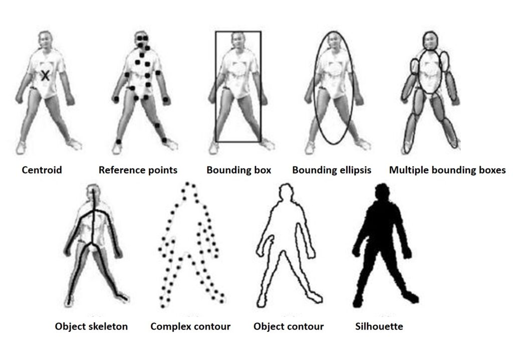
However, among these target representations, the bounding box is by far the most common. The reason for that is that a bounding box can easily define a variety of objects.
The appearance model
So, we saw several ways to represent our target. Now let’s have look at how to model its appearance. The idea behind the appearance model is to describe the target object based on the available visual information. Therefore, a suitable appearance model is a discriminative model.
- Image histogram
For instance, in the image below we can notice a football player wearing a blue uniform running along the field. The player is represented with a bounding box.
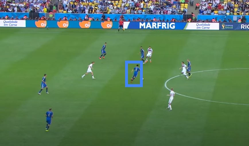
This bounding box will define a histogram. Usually, we use a histogram on a grayscale image but also we can use a color histogram. In the image above we can imagine a color histogram of the rectangular bounding box. We can use this histogram to differentiate the target player from the green background.
Now. let’s illustrate this whit an example. For instance, we can have a histogram that has 70% of blue color and 30% of green color. That means that when the player moves we need to move the bounding box over the area and find the place with the highest percentage of blue color. So, basically by finding a box, we will always have a perfect match with an initial histogram. In that way, we will be able to track the player.
- Image intensity
Also, we can use the reference image itself as an appearance model. In this case, the target object is described as a set of pixel intensities. For example, if the target object is moving, our goal is to find an exact match with the reference image. This process is called template matching. It identifies the region of an image that matches a predefined template. However, the problem in visual tracking is that this image can be warped, rotated, projected, etc. This means that template matching will not work were very well if the image is distorted.

We could also represent a target using a filter bank that computes the resulting image using the original pixel intensity values. We can use distribution fields as the appearance model. These types of appearance models are also called Region-based methods.
- Image features
Another very popular type of appearance model are image features. It is based on the reference image of the target object where a set of distinguishable features can be computed in order to represent the target. To extract the features, several object detecting algorithms are often used. For example, algorithms like SIFT, SURF, ORB, Shi-Tomasi that we reviewed in our post How to extract features from the image in Python.

- Subspace decomposition
In certain cases, the subspace of the reference image is used to model the object’s appearance. These more sophisticated models have proven to be very useful in situations where the appearance of the tracked object varies in time. A Principal Component Analysis and dictionary-based approaches are often employed in this context. Here, the reference image of the target object can be decomposed. For instance, let’s say that we have an image dataset of 100 persons. We will get a mean image and add one component. This component captures a direction whether a person is looking to the left or to the right. Then, we can use this component to search for the people looking to the right.
https://en.wikipedia.org/wiki/Eigenface
Next, we will focus on the types of appearance models, which are often used in Region-based tracking methods.
3. Region-based tracking methods
Region-based tracking comes from the idea of tracking a region or a portion of an image. So as agreed we will represent a target object with a bounding box. In order to track the objects contained within the bounding box, we need to define a suitable appearance model. In the example below, the appearance model is a template intensity image. Here, we have a reference image of the target object on the left, and we are searching for the best match in the original image.
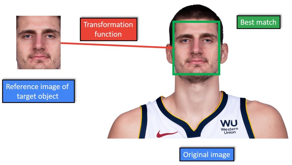
Now that we have adopted an appearance model for our target object, we need to model its motion in the scene. That means that the tracking problem solves the finding of the parameters of the motion model. The parameters of the motion model maximize the similarity between the reference and original image of the target object. For instance, let’s assume that the target object only moves in the horizontal and vertical directions in the scene. In this case, a very simple translational model, with only two parameters \(t_{x} \) and \(t_{y} \) is sufficient to model the position of the reference image.
Naturally, if the target object moves in more complex ways, then we need to adjust and use more complex transformation models with additional degrees of freedom as shown below:
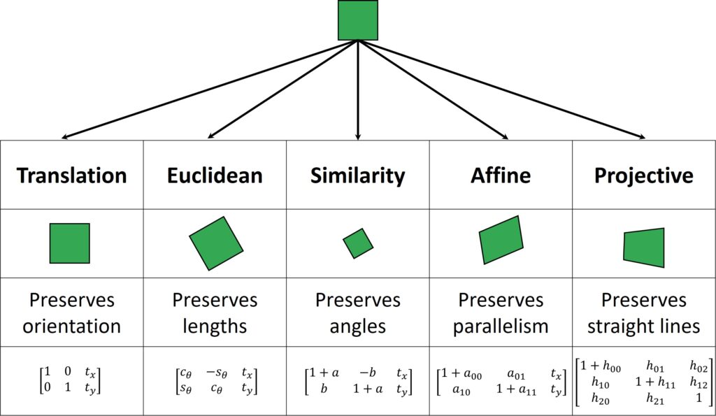
For instance, if we’re tracking a book cover, then we must use a projective model which has eight degrees of freedom. On the other hand, if the target object is not rigid we need to use a deformable model. So, we could use a B-Spline or Thin-Plate Splines to correctly describe the object’s deformation.
Deformable parametric models:
- Splines (B- Splines, TPS, Multivariate )
- Triangular meshes
Another particular aspect of direct methods is that in practice, we often use the positions of the target object in the previous frames to initialize the search for its current position. So, given the parameter vector \(p_{t-1} \) of our motion model at a previous frame, \(t-1 \), our task is to find the new vector \(p_{t} \), which best matches the reference and the current image.
The similarity function
This leads us to a very interesting question. What exactly is the best match for the reference and current image? Well, to find the best match means to find the portion of the current image that is most similar to the reference image. That means we have to choose a similarity function \(f \) between the reference and the original image. This was used in template matching. In the following example, we can see that the similarity between the first two images should be larger than the similarity between the second two images.

To calculate the similarity between template and original image, several similarity functions are used. Here are just a few of them:
Similarity functions:
- Sum of Absolute Differences (SAD)
- Sum of Squared Differences (SSD)
- Normalized Cross-Correlation (NCC)
- Mutual Information (MI)
- Structural Similarity Index (SSIM)
So, we have learned that for tracking we need to choose an appearance model for the target object, a motion model, and a similarity function in order to tell how similar the reference image is to the original image in a video. So, given the parameters \(p_{t-1} \) for the previous frame \(t-1 \), we need to devise a search strategy to find the new model parameters \(p_{t} \) at the current time \(t \). The most simple approach is to define a local area search around the previous parameters \(p_{t-1} \). In the example below, we will move from \(-20 \) pixels to \(+20 \) pixels along the \(x \) axes, and from \(-20 \) pixels to \(+20 \) pixels along the \(y \) axes from the position of the target object in the previous frame (assuming that we have only translation).

If we want to improve an exhaustive search on a wide neighborhood around the object’s previous position, we can reduce our search using our prior knowledge of the object’s motion. For instance, we can use a classical Kalman filtering framework or more sophisticated filters such as the Particle filter.
4. Gradient-based methods
Another very popular search strategy is Gradient descent. First, we choose a similarity function, that is differentiable with respect to the tracking parameters and has a smooth and convex landscape around the best match. Then, we can use gradient-based techniques and find the optimal parameters of the transformation (motion) model.
In the following example, we have the case where we need to calculate the SSD (Sum of Squared Differences).
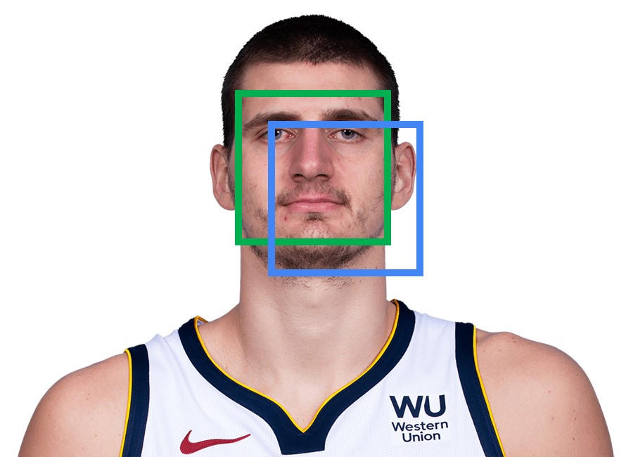
Let’s assume that the green patch is the reference image and that we want to check the similarity with an original image (blue patch). We will calculate SSD by shifting the blue rectangle to match the green rectangle and we will subtract these two images. Then, we will square the differences and sum them up. If we get a small number that means that we have a similar template. This process is illustrated in the following image.

The important thing to note is that SSD will be a function of a vector \(p \), where \(p=\left [ \begin{matrix}x\ y\end{matrix} \right ] \) is a vector. Here, \(x \) and \(y \) are the translation parameters that we are search for. The result of the computation of the SSD score for the blue rectangle, for a plus-minus five-pixel displacement around the optimal place of alignment, gives us this curve. So we can clearly see the convex and smooth nature of the SSD in this example.
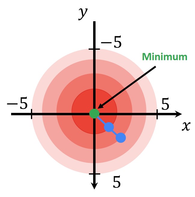
In the example above on the right side, we can see a 2D function from a bird’s perspective. In the center is the minimum and then we have larger values around. Now, if we want to draw this function in 1D it will look like this:
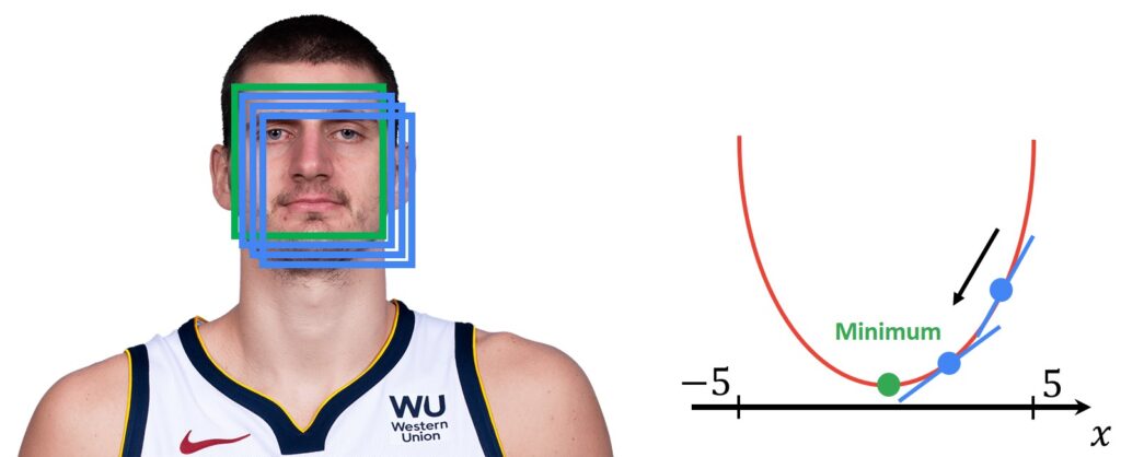
So, let’ say that we search along the \(x \) direction. First, we will randomly choose the starting position for the \(x \). Let’s say \(x=4 \). Then we will calculate the gradient of the SSD function. Next, we will know that we need to move towards the minimum of the function. The gradient will tell us in which direction we need to move in the original image.
So, what is the major advantage of the Gradient descent? Well, imagine we have a transformation model with multiple degrees of freedom, such as the projective model that we’re using to track this board in the following example.
First, let’s explain what multiple degrees of freedom means. Let’s say that we have an original image of the rectangle and a template image. Notice that in the example below the rectangle in the original image on the left side is a projected version of the template image on the right side.
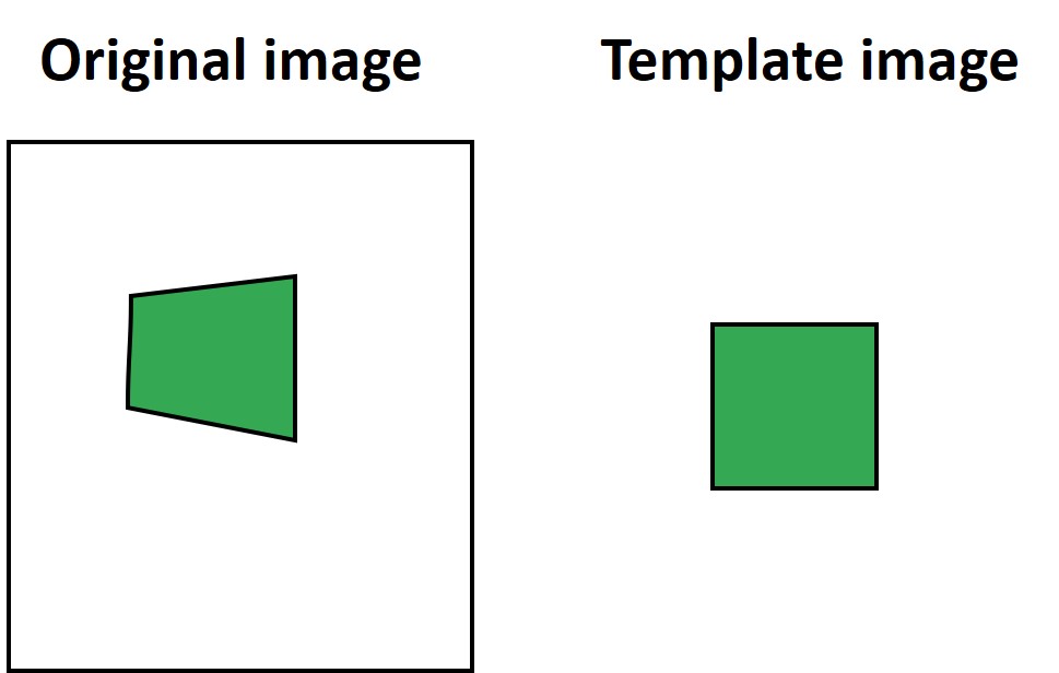
However, now it will be impossible for us to calculate the SSD. One way to solve this problem is to detect keypoints in both images, and then use some feature matching algorithm that will find their matches. However, we can also do the search using template image intensity values. In order to do that we will apply a transformation warping. As we explained earlier in the post, we will multiply the image with the following transformation matrix:
$$ \left[\begin{array}{ccc}1+h_{00} & h_{01} & h_{02} \\h_{10} & 1+h_{11} & h_{12} \\h_{20} & h_{21} & 1\end{array}\right] $$
This means that here we have 8 degrees of freedom because in the matrix we have a total of 8 parameters and one number that is fixed to 1. So, basically, our initial rectangle will now have a change in perspective. This means that to calculate the SSD, apart from finding just translation parameters \(x \) and \(y \), we also need to find other parameters to represent rotation, scaling, skewing, and projection.
So, the major advantage of the Gradient descent is that when an object that we are searching for is rotated, scaled, and warped, we don’t need to search through 1000s and 1000s of combinations in order to find the best transformation parameters. With Gradient descent, we can obtain these parameters with very high accuracy in only a few iterations. So, it’s a major save in computational effort.
Summary
In this post we have learned that image tracking methods are composed of four major components: appearance model, transformation model, similarity measure, and search strategy. We introduced a few appearance models and also we talked about transformation models, both rigid and non-rigid. Furthermore, we also explained how to calculate SSD, and we also explained how to apply Gradient descent – one of the most common search strategies. In the next posts, we will continue to use these methods.
References:
Direct Visual Tracking – Part I – Introduction to visual tracking (Video 1) – YouTube
Direct Visual Tracking – Part I – Introduction to visual tracking (Video 2) – YouTube