*Understanding the fundamental building blocks that power modern AI systems*

—

## The Building Blocks of Neural Networks

One of the most basic blocks that you’re going to have in your toolbox when you build large complicated neural networks is a linear classifier, illustrated here with stacked building blocks showing the layered structure. Much of the intuition and technical bits that we’ll cover today will carry over completely to the neural network systems that we’ll talk about later.

Hands stacking colored blocks with arrows pointing to ‘Linear classifiers’

So sort of speaking coarsely once we move beyond linear classifiers and move to these big complicated neural models, then we’ll see that the individual components of those neural network models will look very similar to these linear classifiers that we’ll talk about today.

## Recall CIFAR10: Our Working Dataset

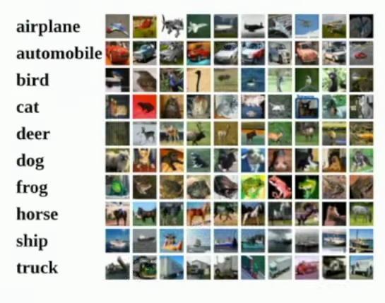
As a quick recap, we’re examining the CIFAR10 dataset. The CIFAR10 dataset is a standard benchmark dataset for image classification containing 50,000 training images and 10,000 test images, organized into 10 distinct categories including airplane, automobile, bird, cat, deer, dog, frog, horse, ship, and truck.

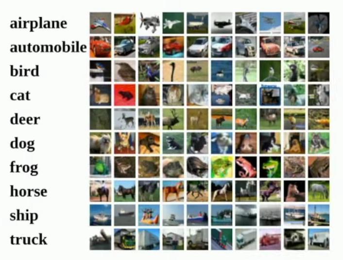
Grid of example images for each category

Each image is 32x32x3 pixels in size. Within each pixel we have three scalar values for the red, blue, and green color channels of the pixel. So the idea of a linear classifier is part of a much broader set of approaches toward building machine learning models.

## Parametric Approach: The Foundation

The parametric approach takes an input image represented as a 32x32x3 array (3072 numbers total) and processes it through a function f(x,W) that outputs 10 numbers representing class scores. The system introduces a new component called parameters or weights (W), shown in red, which are learnable components of the system.

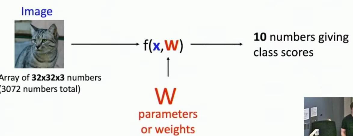
Flow diagram showing image input, function f(x,W), and output scores

The function f(x,W) takes both the image input x and these learnable weights W to produce classification scores for each of the 10 categories. The input image dimensions of 32x32x3 result in 3,072 total scalar values that comprise the pixels of the input image.

And this idea of a parametric classifier will carry over completely to the neural network systems that we’ll talk about. But today we’re going to talk about the possibly the simplest, the simplest possible instantiation of this parametric classifier pipeline.

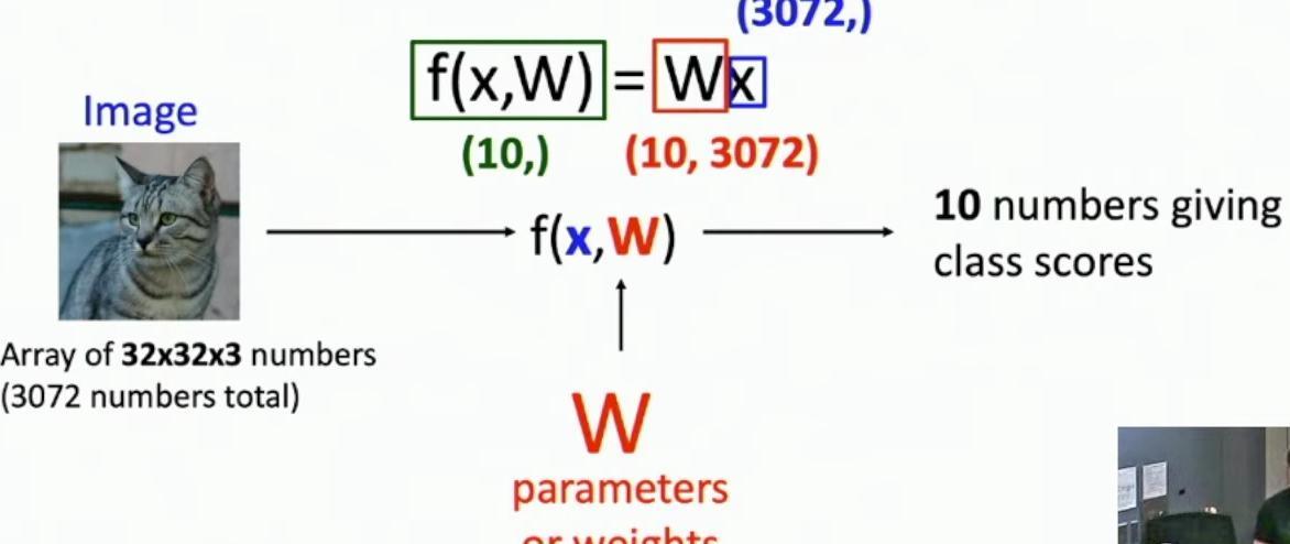
And that’s the linear classifier where it has the simplest possible functional form where this F of image X and weights w is just going to be a matrix vector multiply between the learnable weights w and the pixels of the image X.

## Linear Classifier: Concrete Implementation

The output is a vector of size 10, producing one score for each of the 10 categories that the linear classifier needs to recognize, as shown in the f(x,W) function diagram.

Linear classifier diagram showing image input (32x32x3) to class scores (10) transformation

Linear classifiers can include a bias term B, resulting in a matrix vector multiply plus an offset vector with 10 elements – one for each category being learned. This linear classifier approach can be understood through the lens of image classification, which we’ll explore in subsequent slides.

Let’s examine a concrete example using the shown 32x32x3 image array (3072 numbers total) being transformed by the weight parameters W into 10 class scores.

## Example for 2×2 Image, 3 Classes (Cat/Dog/Ship)

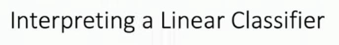
Suppose that our input image is a 2×2 grayscale image of a cat, containing four pixel values: 56, 231, 24, and 2. The pixels are then stretched out into a column vector with four entries, transforming from a (2,2) matrix to a (4,) vector.

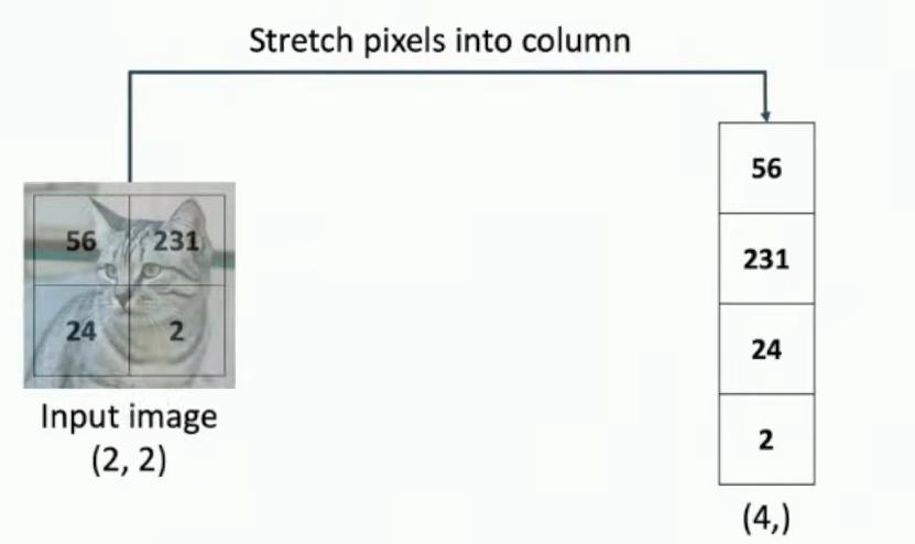
2×2 grayscale cat image with labeled pixel values

The resulting column vector contains the values [56, 231, 24, 2] in order from top to bottom. For this example, we’ll consider classifying only three categories (cat, dog, and ship), using the function f(x,W) = Wx + b.

In this example for classifying cats, dogs, and ships, the weight matrix W has shape 3 by 4, where 3 represents these three categories and 4 corresponds to the total pixels in our 2×2 input image. The bias vector b has shape (3,) to match the three categories, with specific values of 1.1, 3.2, and -1.2 for each class.

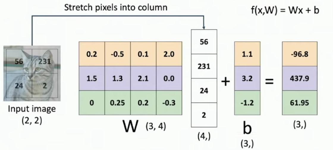
Matrix multiplication diagram showing W(3,4) dimensions

After performing the matrix multiplication f(x,W) = Wx + b, we output a vector of scores with shape (3,) containing values -96.8, 437.9, and 61.95 for each category.

## Understanding the Structure

Looking at the problem this way reveals how we structure image classification by stretching the 2×2 input pixels into a column vector [56, 231, 24, 2]. Each row in the weight matrix W corresponds to one category, with the first row [0.2, -0.5, 0.1, 2.0] for cats, second row [1.5, 1.3, 2.1, 0.0] for dogs, and third row [0, 0.25, 0.2, -0.3] for ships.

So I think it’s useful to think about linear classifiers in a couple of different equivalent ways. And when you think, and by using different viewpoints to think about linear classifiers, it can make certain properties of them very obvious or non-obvious. So having different ways to think about a linear classifier can help you understand it more intuitively.

## The Algebraic Viewpoint

The first way to think of linear classifiers is the algebraic viewpoint, demonstrated here with the function f(x,W) = Wx + b, showing matrix multiplication plus a vector offset. And if you think about the algebraic viewpoint of a linear classifier, there’s a couple of features or facts about linear classifiers that immediately become obvious.

## Linear Classifier: Bias Trick

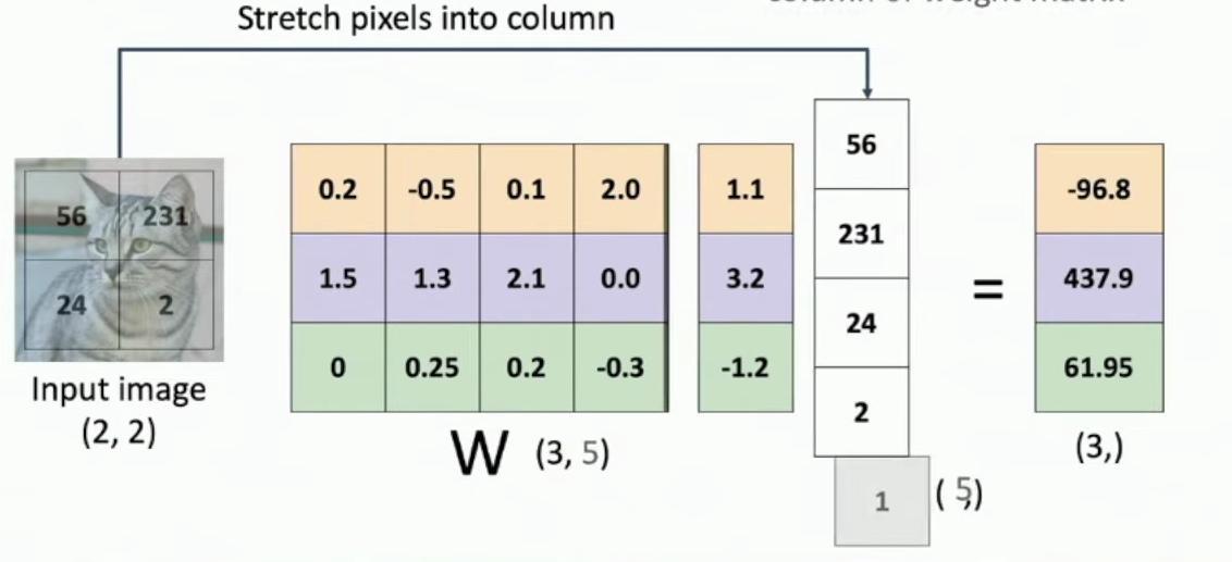
The bias trick incorporates the bias directly into the weight matrix W by augmenting the input vector with a constant 1 and adding an extra column to W. The input image pixels are stretched into a column vector of size (5), where the last element is the appended constant 1.

Matrix multiplication diagram showing input image transformation

The weight matrix W is augmented with an additional column containing values (1.1, 3.2, -1.2) that absorb the bias terms.

## Practical Considerations: The Bias Trick

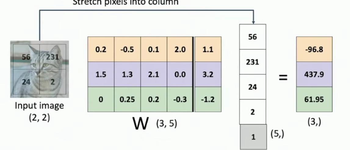
The linear classifier implements a bias trick where we add an extra 1 to the data vector (making it a 5-element column), and the bias is absorbed into the last column of the weight matrix W (3,5), as shown in the matrix multiplication example with the cat image input. This bias trick is pretty common to use when your input data has a native vector form.

Matrix multiplication diagram showing cat image input and weight matrix

But in fact, in computer vision, this bias trick is less common to use in practice because it doesn’t carry over so nicely as we move from linear classifiers to convolutions later on. And furthermore, it’s nice sometimes to separate the weight matrix W (3,5) from the bias into separate parameters for different initialization or regularization approaches.

## Linear Predictions: A Key Property

Another thing that’s very obvious when you think about linear classifiers in this algebraic way is that the predictions are linear, as shown by the fundamental equation f(x,W) = Wx. When we ignore the bias and scale our whole input image by some constant c, we can pull that constant out of the linear classifier, as demonstrated by the equation f(cx,W) = W(cx) = c * f(x,W).

And that means that the predictions of the model will also be scaled by that scalar value c. So if you think about images, that means that if we have some original image on the left with some predicted cat classifier scores from a linear classifier, then if we were to modify the image by desaturating it, by multiplying all the pixels by one half, then all of the predicted category scores from the classifier would all be cut in half as well.

But somehow it’s unintuitive that scaling down all the pixels changes the predicted scores from 437.8 to 218.9 for the middle class, and similarly halves the other scores from -96.8 to -48.4 and 62.0 to 31.0.

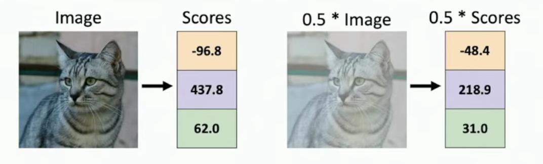
Score comparison between original and scaled images

So this is maybe a bug, maybe a feature, but it feels kind of weird for linear classifiers to behave linearly, where f(x,W) = Wx, as shown by the mathematical relationship. Because you might think that just by scaling down all the pixels by a constant value of 0.5, we can still recognize this as a cat just as easily, as demonstrated in the example images.

## Interpreting Linear Classifiers: Visual Viewpoint

The algebraic viewpoint of linear classifiers can be expressed as f(x,W) = Wx + b, which forms the fundamental equation for classification. But we can reformulate this computation in an equivalent but slightly different way that will give us a slightly different way to think about exactly what linear classifiers are doing in the context of image data.

Linear classifier equation f(x,W) = Wx + b

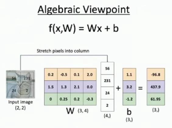
In the algebraic viewpoint, the classification score for each category is calculated through matrix multiplication, where W is a 3×4 weight matrix multiplied by the input vector, plus a bias term b. In this algebraic viewpoint, we take the pixel values of our 2×2 input image and stretch them into a column vector of length 4, as shown in the diagram.

Rather than stretching out the image into a column vector of size (4,1) as shown in the diagram, we can instead think about reshaping the rows of the W matrix (3,4) into the same shape as the input image (2,2).

So here, we’ve taken each of the rows of the matrix W (3×4) and reshaped them into 2×2 blocks that match the dimensions of our input image (2,2). The rows of matrix W are organized into three 2×2 blocks with specific values: one in peach (0.2, -0.5, 0.1, 2.0), one in purple (1.5, 1.3, 2.1, 0.0), and one in green (0, 0.25, 0.2, -0.3).

Matrix W breakdown with color coding

When we interpret linear classifiers from this algebraic viewpoint, using f(x,W) = Wx + b, we can better understand how the weight matrix W and bias vector b interact with the input image.

## Visual Viewpoint: Template Matching

So that’s what I like to call the visual viewpoint of linear classifiers, which we can see demonstrated through a dataset of 10 image categories including airplanes, automobiles, birds, and other objects. And this interpretation of a linear classifier looks kind of like template matching, where each category is associated with a specific weight pattern.

Grid of images showing 10 categories: airplane, automobile, bird, cat, deer, dog, frog, horse, ship, truck

A linear classifier learns one template per category to recognize, as shown in the weight matrices (W) and bias values (b) for different classes. To produce the category score, the classifier computes an inner product between the template weights and the input image pixels, followed by adding the bias term.

The learned templates can be visualized as images themselves, as shown in the bottom row of category-specific templates, providing intuition about what features the linear classifier seeks in each category.

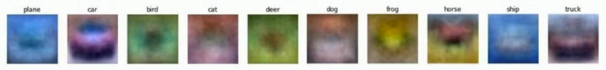
Row of learned template visualizations for different categories

Looking at these visualizations, we can see each category template captures characteristic features – for instance, car, bird, cat, deer, dog, frog, horse, ship, and truck each have distinct color patterns and shapes. Images with color patterns matching these templates will receive higher scores for their respective categories. The templates show how each class learns to recognize both object features and contextual background patterns.

And one thing that’s kind of interesting from this viewpoint is that it becomes clear that even though we told the classifier that we wanted to recognize object categories, like planes and dogs and deer, in fact, it’s using a lot more evidence from the input image than just the object itself. And it’s in fact relying very strongly on the context cues from the image. So, right, if you, so for example, if you imagined putting in an image that had a deep, that had maybe a car in a forest, that would be kind of confusing for a linear classifier.

## Understanding Linear Classifier Limitations

Linear classifiers have one template per category, as demonstrated by the blurred template images for different object classes like car, bird, cat, and others. The visual viewpoint of interpreting linear classifiers reveals how they process and classify images, as shown by the weight matrices (W) and bias values (b) for different categories.

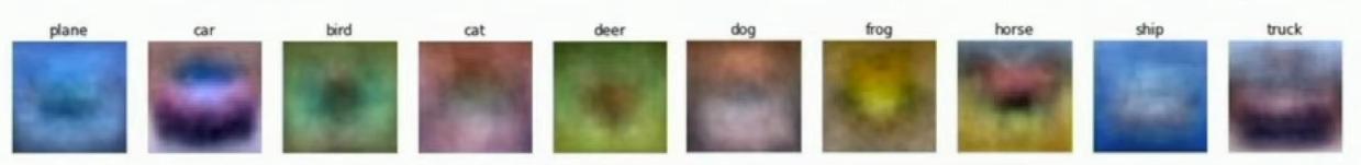
Row of blurred template images for different object categories

And that becomes very obvious when you think about the visual viewpoint of these linear classifiers. So another potential failure mode of linear classifiers that becomes clear when you think about this visual viewpoint is that of mode splitting.

So our linear classifier is only able to learn one template per category, but there’s a problem. What happens if we have categories that might appear in different types of ways? So as a concrete example, think about horses. So if you go and look at the CFR-10 dataset, which maybe you might have done if you started working on the first homework assignment, then you’ll see that horses on CFR-10 are sometimes looking to the left, and they’re sometimes looking to the right, and they’re sometimes looking dead on.

Now, if we have horses that are looking in different directions, then the visual appearance of the images of horses looking in different directions will be very different. But unfortunately, the linear classifier has no way to disentangle its representation and no way to separately learn templates for horses that are looking in different directions.

So in fact, if you look at this example of a, if you look at this learned template of a horse from this one particular linear classifier, you can kind of see that it actually has two heads. So if you look at the horse here, he has kind of a brown blob in the middle and green on the bottom, which you might expect. But now there’s a black blob on the left and a black blob on the right, which might court.

So then this is the linear classifier, trying to do the best that it can to match horses looking in different directions, using only a single template that it has the ability to learn. So this is also somewhat visible in the car example. You can see that the car template doesn’t actually look anything like a car. It just kind of looks like a red blob and a windshield.

And again, the car template might have this funny shape because it’s trying to use a single template to cover all possible appearances of cars that you might see in the data set. This also gives us a sense that maybe C410 has a lot of red cars because the car template that’s learned is red. And maybe if we try to recognize green cars or blue cars, then the classifier might fail.

And all of these type of failure modes become very obvious when you think about the linear classifier from this visual viewpoint.

## Geometric Viewpoint: Understanding High-Dimensional Spaces

So another third way that we can think about linear classifiers is what I like to call the geometric viewpoint. Looking at the graph, we can see how classifier scores for airplane, deer, and car categories vary linearly as we change the value of pixel (15, 8, 0), while keeping all other pixels fixed in the image.

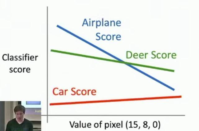
Linear plot showing three classifier scores vs pixel value

The classifier score must vary linearly as we change any individual pixel value, which is demonstrated by the straight-line relationships in the graph for airplane, deer, and car scores. So this example becomes more interesting when we look beyond a single pixel (15, 8, 0) and consider how the classifier scores for airplanes, deer, and cars vary across pixel values.

We can broaden this viewpoint by incorporating multiple pixels simultaneously, as shown by the 32x32x3 array containing 3072 total numbers for image classification. So then we can imagine drawing a plot where the x-axis and y-axis represent different pixel coordinates, as shown with the points (11,11,0) and (15,8,0).

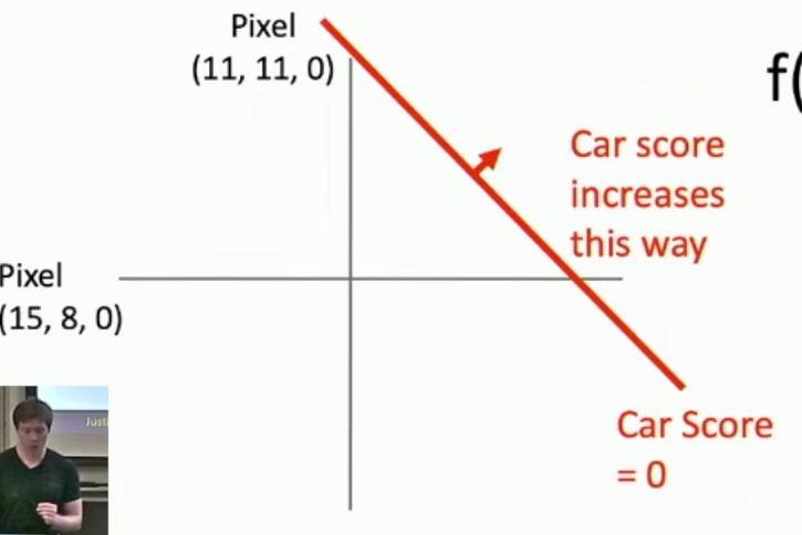
2D plot showing pixel coordinates and car score line

The diagram shows a 2D representation where we can visualize how the car score changes across different pixel values. The line shown in the diagram represents where the car score equals zero. This level set of the car score forms a line in this pixel space, with an arrow indicating the direction of increasing car scores.

The car score increases linearly in a direction orthogonal to this line, as indicated by the red arrow labeled ‘Car score increases this way’. The car template will lie somewhere along this line which is orthogonal to the level set of the car score.

For all the different categories we are trying to recognize, we’ll have different lines with different level sets, with the learned templates for those categories orthogonal to their respective level sets. Looking at only two pixel images like in this example is not very intuitive, especially when dealing with actual 32x32x3 arrays containing 3072 numbers total, as shown with the cat image example.

But you can imagine that this viewpoint would extend to higher dimensions as well. The linear classifier f(x,W) = Wx + b takes the whole space of images as this very high-dimensional Euclidean space. And now within that Euclidean space, we have different hyperplanes that are trying to one hyperplane per category that we want to recognize.

Each of the hyperplanes for each of the categories we want to recognize are now cutting this high-dimensional Euclidean space into two half spaces along this level set. The geometric viewpoint of linear classifiers shows how one hyperplane per class divides the high-dimensional space, as illustrated by the airplane, car, and deer score lines intersecting in different dimensions.

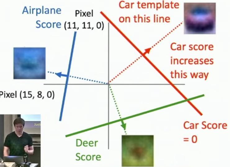
2D plot showing score lines for airplane, car, and deer classifications

## The Challenge of High-Dimensional Geometry

While this geometric viewpoint provides useful insights into linear classifiers, as shown by the pixel score coordinates and classification boundaries, geometry becomes increasingly complex in higher dimensions. So we unfortunately are cursed to live in a low-dimensional, three-dimensional universe.

So all of our physical intuition about how geometry behaves is really shaped by these very low number of dimensions. The behavior of Euclidean geometry in high dimensions, as shown in the 3D hyperplane visualization, can be very different from our low-dimensional experience.

While the geometric viewpoint illustrated by these classification boundaries and score lines is useful, it must be approached with caution. It’s very easy to be led astray by geometric intuition because we happen to have all our intuition built on low-dimensional spaces.

## Hard Cases for Linear Classifiers

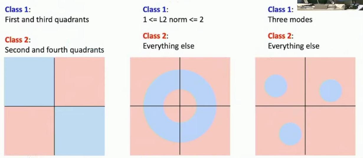
The slide titled ‘Hard Cases for a Linear Classifier’ introduces three challenging classification scenarios that are impossible for linear classifiers to properly recognize. The slide presents three two-dimensional spaces where red and blue regions correspond to different classification categories, illustrating cases where linear classification fails.

Three diagrams showing classification scenarios with red and blue regions

The first example shows quadrant-based classification, where Class 1 occupies the first and third quadrants while Class 2 covers the second and fourth quadrants. The middle example shows a circular pattern where Class 1 is defined by points with L2 norm between 1 and 2, while Class 2 encompasses everything else. The third example shows a three-mode pattern where Class 1 consists of three distinct circular regions separated by Class 2.

And then if you think about it, there’s no way that we can draw a single hyperplane that can divide this, that can divide the red and the blue here. So that’s a case that is just impossible for linear classifiers to recognize. Another case that’s completely impossible for linear classifiers is this case on the right, which is very interesting, of three modes.

So here, this, here we’ve got the blue in the blue category, there’s maybe three distinct patches and parts in regions in pixel space that correspond to possibly different visual appearances of the category where we wish we want to recognize. And then if we have these different disjoint regions in pixel space corresponding to a single category, again, you can see there’s no way for a single line to perfectly carve up the red and the red and the blue regions.

So this, this, this right example of these three modes is, I think, similar to the, what we saw in the visual example of maybe the horses looking in different directions that you can imagine, maybe in this high-dimensional pixel space, there’s some region of space corresponding to horses looking right and a completely separate region of space corresponding to horses looking in a different direction.

And again, with a single, and now with this geometric viewpoint of hyperplanes cutting up high-dimensional spaces, it again becomes clear that there’s, it’s very difficult for linear classifier to carve up classes that have completely separate modes of appearance.

### Historical Context: The Perceptron

And this also ties back to the historical context that we saw in the first lecture. If you remember, in the first lecture last week, we talked about this historical context of different types of machine learning algorithms people had built over the years. And one of these very first machine learning algorithms that got people very excited was the perceptron.

That all of a sudden there was this machine that could learn for data, it could learn to recognize digits and characters and got people really excited. But it had this, but now if we were to, if you were to look back at the exact math of the perceptron now, we would recognize it as a linear classifier. And because the perceptron was a linear classifier, there’s a lot of things that was just fundamentally unable to recognize.

The most famous example was the X-Worf function, which is shown here, which where we have the green is one category and the blue is a different category. So because the linear, because the perceptron was a linear model.

## Summary: Three Viewpoints of Linear Classifiers

So then, to this point, we’ve talked about linear classifiers from an algebraic viewpoint, represented by the equation f(x,W) = Wx, which involves a matrix-vector multiplication. We’ve seen how this simple equation can be understood from three distinct viewpoints: algebraic (matrix multiplication), visual (template matching with one template per class), and geometric (hyperplanes cutting up space).

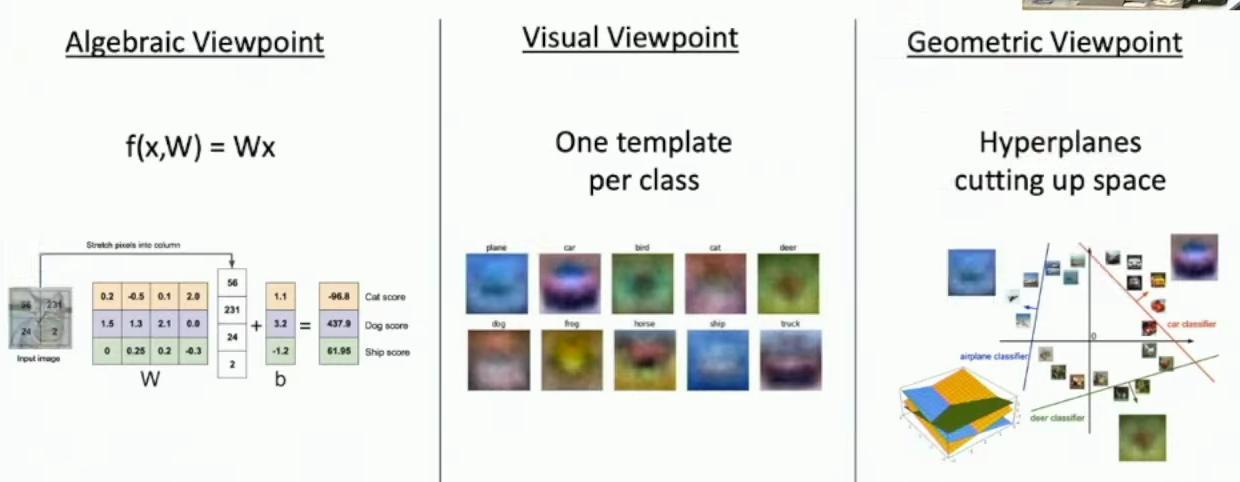
Three-panel comparison showing algebraic, visual, and geometric viewpoints

## Moving Forward: The Need for Loss Functions

So far, we have defined a linear score function f(x,W) = Wx + b that can compute class scores for an image x. Given any value of the weight matrix W, we can compute class scores for input images, as demonstrated in the scoring table showing values for different object categories.

Three images with corresponding score matrix for 10 categories

Here we have three example images – a cat, a red sports car, and a tree frog – with scores computed across 10 categories including airplane, automobile, bird, and others. For any particular value of W, we can compute score vectors, as shown in the numerical table where scores range from -8.87 to 6.14 across different categories.

But how can we actually choose a good W? We’ve not said anything about the learning process by which this matrix W is selected or learned from data. So now, in order to actually implement linear classifiers, we need to talk about two more things.

We need to use a loss function to quantify how good a value of W is, as shown in the mathematical function f(x,W) = Wx + b. And that’s what we’ll talk about for the rest of this lecture. In the next lecture, we’ll focus on optimization to find a W that minimizes the loss function, searching across all possible values to find the optimal solution for our training data.

## Introduction to Loss Functions

A loss function tells how good our current classifier is, with a direct relationship to its performance. Low loss indicates a good classifier, while high loss indicates a bad classifier. And the whole goal of machine learning is to write down a loss function, well, OK, that’s a little bit reductive.

But one way that we can think about a lot of neural network systems is writing down loss functions that try to capture intuitive ideas about what types of models or when models are working well, and when models are not working well. And then once we have this quantitative way to evaluate models, then to try to find models that do good.

The loss function is also known by alternative names: objective function and cost function. And because people can never agree on names, sometimes people will talk about the negative of a loss function instead. So then with loss function is something you want to minimize. Sometimes people want to maximize something instead.

This concept is also known as an objective function or cost function, and when expressed negatively, it can be called a reward function, profit function, utility function, or fitness function. It’s just a way to quantify what your model is doing well and when your model is not doing well.

So, a bit more formally, the way that we’ll usually think about this is we have some data set of examples where each input is a vector x and each output is a label y. In the image classification case, x will be these images of fixed size and y will be an integer giving the label, will be an integer indexing into the categories that we care to recognize.

Now, the loss for a single example will often write as Li and it will take in, so then f of xi and w will be the predictions of our model on a data point xi and the loss function will then assign a score of badness between the prediction and the ground truth or true label yi. And then the loss over the entire data set will simply be the average of all the losses of the individual examples in the data set.

So then this is kind of the idea of a loss function in the abstract and the first concrete loss function. And then you can imagine that as we try to tackle different tasks in machine learning, we need to write down different types of loss functions for each different task that we want to try to solve. And even when we’re focused on a single task, we can often write down different types of loss functions that encapsulate different types of preferences over when models are going to be good and when models are going to be bad.

So as a first example of a loss function, I want to talk about the multi-class SVM loss for image classification or really for classification more generally.

—

*This concludes Part 1 of our exploration into Neural Networks and Linear Classifiers. In this foundational piece, we’ve covered the essential building blocks of deep learning – from the basic parametric approach to the three key viewpoints for understanding linear classifiers: algebraic, visual, and geometric. We’ve also examined the fundamental limitations of linear classifiers and introduced the critical concept of loss functions that enable machine learning systems to learn from data. Part 2 will dive deeper into specific loss functions, optimization techniques, and the mathematical foundations that power modern neural networks.*