dH #025 Image Segmentation Fundamentals: From Point Detection to Advanced Edge Linking
Mastering Image Segmentation Fundamentals: From Point Detection to Advanced Edge Linking
🎯 What You’ll Learn
In this comprehensive guide, we’ll explore the fundamental techniques of image segmentation and edge detection that form the backbone of modern computer vision. You’ll understand the mathematical foundations of derivatives in image processing, master point and line detection methods using second-order derivatives, learn how to implement sophisticated edge detection algorithms including the Canny detector, and discover how to link edges together using both local and global methods. By the end, you’ll have a solid grasp of how these techniques work together to partition images into meaningful regions.
Tutorial Overview
- Course Overview and Basic Concepts
- Finite Differences for Image Processing
- Point Detection Methods
- Line Detection Techniques
- Basic Edge Detection Approaches
- Canny Edge Detection Algorithm
- Edge Linking Strategies
1. Course Overview and Basic Concepts
Introduction to Image Segmentation
Welcome to the world of image segmentation fundamentals! This comprehensive exploration covers several key techniques that form the foundation of computer vision and image processing. We’ll journey through point detection, line detection, and edge detection methods, concluding with image thresholding techniques. This material corresponds to Chapter 10, sections 10.1 through 10.3 of standard computer vision textbooks.
Key insight: Image segmentation is essentially about partitioning an image into meaningful regions or objects, and the techniques we’ll cover are fundamental building blocks for this process.
Image segmentation builds upon fundamental concepts of spatial filtering and convolution. Point detection helps us identify isolated features or anomalies in an image, while line detection allows us to find linear structures and boundaries. Edge detection enables us to locate significant transitions in intensity that often correspond to object boundaries. Finally, image thresholding provides a powerful method for separating objects from backgrounds based on intensity values.
💡 Mathematical Framework
Let us assume we have image \(I\), where \(I\) represents the entire spatial domain or region of the image. Image segmentation is the process of dividing this image \(I\) into several partitions \(R_1, R_2, \ldots, R_n\). These partitions must satisfy several fundamental properties:
- Union Property: All regions together must cover the entire image: \(\bigcup_{i=1}^{n} R_i = I\)
- Connectivity: Each individual region \(R_i\) is a connected set for \(i=1,2,3,\ldots,n\)
- Disjoint Property: There is no overlap between different regions: \(R_i \cap R_j = \emptyset\) for \(i \neq j\)
- Intra-region Similarity: If \(Q\) is a logical predicate for segmentation, then \(Q(R_i) = \text{TRUE}\) for all segments
- Inter-region Dissimilarity: \(Q(R_i \cup R_j) = \text{FALSE}\) for \(i \neq j\)
🔴 Two Fundamental Approaches
Discontinuity-Based Segmentation: Boundaries of regions are sufficiently different from each other and from the background. Edge-based segmentation is a prime example of this approach.
Similarity-Based Segmentation: You partition an image into regions that are similar according to predefined criteria. Region-based segmentation exemplifies this method.

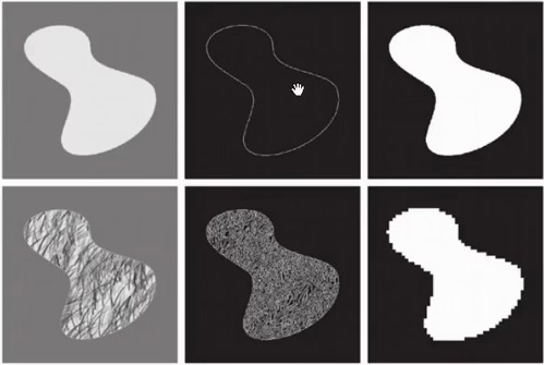
Consider an image with a blob where the inside has constant intensity and the background also has constant intensity. For discontinuity-based segmentation, we identify the boundary between these regions. In a more complex case where the blob has internal texture that’s uniform across the object but differs from the background texture, edge detection operators like gradients or Laplacians reveal that the background shows no intensity differences, while the textured object contains variations due to internal structure. This demonstrates how we need robust methods to detect boundaries and edges for successful object segmentation.
2. Finite Differences for Image Processing
Derivative Properties and Requirements
When working with derivative computation for image processing, we need to understand that first and second order derivatives have distinct characteristics. For first order derivatives, there are three key requirements:
- They must be zero in areas of constant intensity
- Non-zero at the onset of an intensity step or ramp
- Non-zero along intensity ramps
Second order derivatives have slightly different characteristics – they must be zero in areas of constant intensity, non-zero at both the onset and end of an intensity step or ramp, and zero along intensity ramps.
💡 Numerical Derivative Formulations
To estimate derivatives numerically, we have several formulation approaches:
First Order Derivatives:
- Forward difference: \(f'(x) = f(x+1) – f(x)\)
- Backward difference: \(f'(x) = f(x) – f(x-1)\)
- Central difference: \(f'(x) = \frac{f(x+1) – f(x-1)}{2}\)
Second Order Derivatives:
Second order central difference: \(f”(x) = f(x+1) – 2f(x) + f(x-1)\)
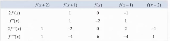
The central difference formulation has a denominator of two because we’re calculating the difference between values of two pixels that are two pixels apart, positioned on either side of the central pixel. These central difference formulations can be extended to calculate higher order derivatives as well.
🔴 Critical Differences Between First and Second Derivatives
First derivatives typically produce thicker edges in images, while second order derivatives have a stronger response to fine details such as thin lines, isolated points, and noise.
An important property of second order derivatives is that they produce double edge responses at ramp and step transitions, which proves useful for locating edges precisely. Additionally, the sign of the second order derivative can indicate whether there’s a transition from dark to light or light to dark regions.
Practical Application Examples
When applied to images, these derivative properties become immediately apparent. Let’s extend the second-order central difference to practical image processing. The second derivative of function \(f\) at location \(x\) is calculated as \(f(x+1) – 2f(x) + f(x-1)\).
$$\frac{\partial^2 f(x)}{\partial x^2} = f”(x) = f(x+1) – 2f(x) + f(x-1)$$
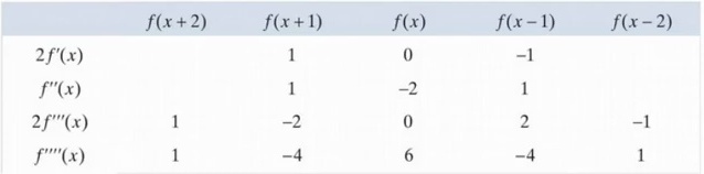
The behavior of first and second derivatives reveals distinct characteristics that make them suitable for different edge detection tasks. First derivatives typically produce thick edges when applied to images, while second derivatives demonstrate a much stronger response to fine details. The double-edge response of second derivatives at ramp and step transitions proves particularly useful for precise edge localization.

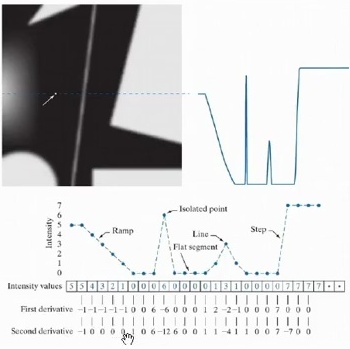
Consider analyzing a linear profile through a sample image that contains various intensity features – ramp-like intensity changes, bright isolated points, roof-shaped edges, and sudden step transitions. By applying derivative equations to calculate both first and second-order derivatives along this profile, we can verify the theoretical properties. For intensity ramps, the first derivative produces non-zero values, while regions of constant intensity yield zero values. At locations of rapid intensity changes, we observe significant responses in the first derivative. The second derivative produces zero values for intensity ramps, which is exactly what theory predicts.
3. Point Detection Methods
The Laplacian Operator Foundation
Point detection leverages second-order derivatives for detecting isolated points in images. The Laplacian operator provides a powerful mathematical foundation for this task by measuring how much a pixel differs from its immediate neighbors.
Mathematical Definition
The Laplacian is defined as the sum of second-order partial derivatives with respect to both the horizontal and vertical axes in the image:
$$\nabla^2 f = \frac{\partial^2 f}{\partial x^2} + \frac{\partial^2 f}{\partial y^2}$$
When we apply a central difference formulation to discretize this continuous operator, we get:
$$\nabla^2 f(x,y) = f(x+1,y) + f(x-1,y) + f(x,y+1) + f(x,y-1) – 4f(x,y)$$
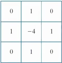
This mathematical formulation can be elegantly represented as a \(3 \times 3\) convolution kernel. The kernel encodes the weights from our discrete Laplacian equation, with the central coefficient being \(-4\) and the neighboring coefficients being \(1\).
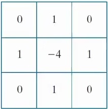
To compute the Laplacian of an entire image, we simply perform a convolution operation between this \(3 \times 3\) kernel and the input image. The resulting value at any given point represents the Laplacian response at that location.
💡 Point Detection Algorithm
The Laplacian operator method follows three essential steps:
- Compute Laplacian: Calculate the convolution between the \(3 \times 3\) kernel and the image at every pixel
- Take Absolute Value: Since the Laplacian can be either positive or negative, we only care about detecting locations of isolated points regardless of sign
- Apply Threshold: If the result is greater than threshold \(T\), set that pixel to \(1\), otherwise set it to \(0\)
This process is expressed mathematically as:
$$g(x,y) = \begin{cases} 1 & |\nabla^2 f(x,y)| \geq T \\ 0 & \text{otherwise} \end{cases}$$
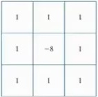
Any location in \(g(x,y)\) with a value of \(1\) indicates an isolated point, while locations with \(0\) are not isolated points. The kernel we use here is isotropic, meaning it calculates the Laplacian not only along horizontal and vertical axes but also along diagonal directions, providing more comprehensive point detection.

🔴 Real-World Application
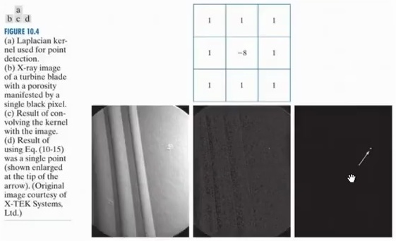
Industrial Defect Detection: A practical example demonstrates this technique using an X-ray image of a turbine blade containing a defect. When we calculate the Laplacian, we eliminate all regions of constant intensity, leaving behind areas where intensity changes rapidly. The processed result shows a brighter dot at the location of the defect. By applying a properly defined threshold, we can isolate this point further and clearly identify the defect location.
4. Line Detection Techniques
Second-Order Derivatives for Line Detection
When it comes to line detection in images, we can leverage both first and second-order derivatives, but second-order derivatives offer distinct advantages. Using the second-order derivative results in a stronger filter response and produces thinner lines compared to first-order derivatives, making it particularly effective for precise edge detection.
Key advantage: The process begins with calculating the Laplacian of the original image using any of the standard kernels we’ve discussed previously for Laplacian computation.
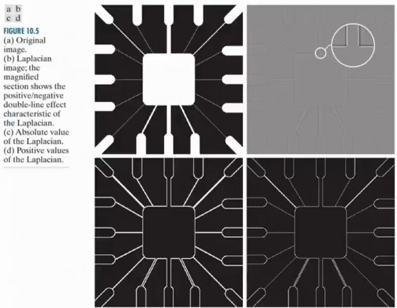
The Laplacian operation reveals an interesting characteristic at line locations – we observe regions of both positive and negative values, creating what appears as a double line effect that marks the location of edges. This dual-polarity response is a fundamental property of second-order derivatives when applied to edge detection.
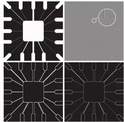
💡 Processing Options for Line Refinement
To refine our line detection results, we have several processing options:
- Absolute Value: Taking the absolute value of the Laplacian produces edges that appear quite thick, which may not be ideal for precise line detection
- Positive Threshold (Recommended): Apply a threshold of zero and work only with the positive values from the Laplacian operation. This selective thresholding technique produces remarkably thin and well-defined lines that accurately represent the location of edges
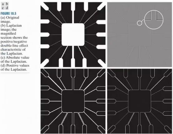
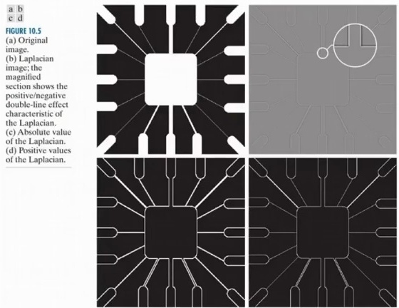
Directional Filter Kernels
Detecting Lines at Specific Orientations
What if we want to locate lines that are not only in horizontal and vertical directions? We can use modified kernels to achieve this goal. Here is a set of four kernels for different orientations:
- Horizontal lines detection
- \(+45°\) angle detection
- Vertical lines detection
- \(-45°\) angle detection
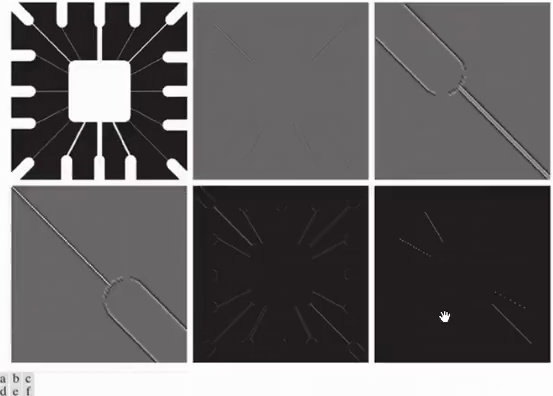
Let’s examine a practical example where our goal is to detect diagonal lines in the direction of positive \(45°\). We apply the corresponding kernel to the image through convolution, and the result shows how effectively this directional filter responds to lines matching that specific orientation.
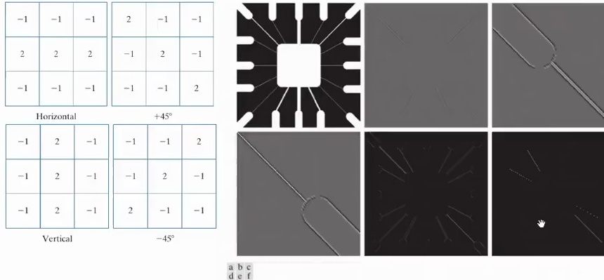
🔴 Threshold Selection for Directional Detection
Critical technique: To refine our results, we can apply a threshold to the convolved image. When we set the threshold value to \(T = 254\) (the maximum pixel value minus 1), we obtain an image where only the edges very close to the \(45°\) direction are highlighted in white. This thresholding operation with the condition \(g > T\) effectively isolates the most prominent diagonal features while suppressing weaker responses and noise.
5. Basic Edge Detection Approaches
Understanding Edge Types in Digital Images
Edge detection is a fundamental approach for image segmentation that relies on identifying local intensity changes and discontinuities within images. Understanding the different types of edges is crucial for selecting the appropriate detection method.
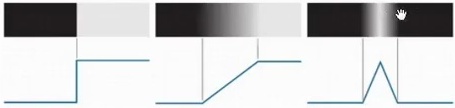
Three Types of Edges
Step Edges: Sharp transitions between two intensity levels that ideally occur over the distance of just one pixel, creating an abrupt change in brightness.
Ramp Edges: Feature a gradual transition between two intensity levels, where the change occurs smoothly over several pixels.
Roof Edges: Present a unique pattern where the intensities on both sides are similar, but there’s a distinctly different intensity value in the middle, creating a peak-like or valley-like structure.
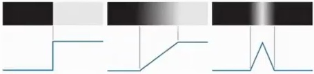
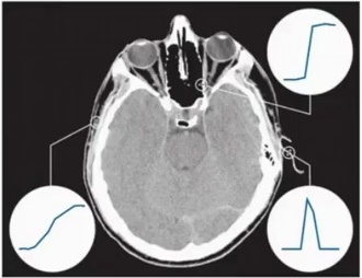
When we examine real medical images, such as brain scans, we can observe these edge types in practical applications, though they rarely appear as perfectly as in theoretical examples. In actual brain imagery, we might find rough approximations of ramp edges where there’s a smooth transition between different tissue types, examples of roof edges at anatomical boundaries, and approximate step edges at sharp structural interfaces.
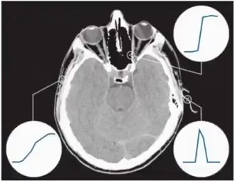
💡 Mathematical Approach to Edge Detection
The mathematical approach involves using derivatives to identify intensity changes:
- First Derivative: Produces thick edges in images
- Second Derivative: Creates a double edge profile characterized by a sign change – one positive spike followed by a negative spike
The double edge profile is particularly useful because we can locate the exact edge position by finding where the line crosses zero between these two spikes. For a ramp edge, the first-order derivative will be non-zero throughout the ramp region and zero outside it, while the second-order derivative shows the characteristic double spike pattern.
🔴 The Noise Challenge
Critical consideration: A critical issue in edge detection is the impact of noise on derivative calculations. When we add Gaussian noise with zero mean and standard deviation of \(\sigma = 0.1\) to an ideal ramp edge, the noise may not be immediately visible in the original image. However, both first and second-order derivatives show significantly increased sensitivity to this noise because they calculate differences between neighboring pixels, which amplifies the noise effects.
This magnification occurs because derivative operations inherently enhance high-frequency components in the signal, and noise typically contains high-frequency information. The result is that even small amounts of noise become much more prominent in the derivative calculations, making noise reduction an important preprocessing step.
Zero-Crossing Methods
Precise Edge Localization
Zero-crossing methods represent a fundamental approach that leverages the mathematical properties of derivatives to precisely locate edges in digital images. The core principle lies in analyzing how the first and second derivatives of an image’s intensity function behave at edge boundaries.
When we examine an ideal edge – essentially a transition between two regions of constant intensity – the first derivative produces a thick edge profile that spans multiple pixels, making it difficult to pinpoint the exact edge location with high precision.
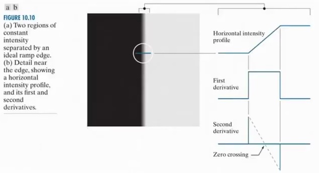
The real power of zero-crossing methods emerges when we consider the second derivative of the intensity function. Unlike the first derivative’s broad response, the second derivative produces a distinctive double-edge profile characterized by a crucial sign change at the edge location. This sign change manifests as a zero-crossing point that corresponds precisely to the edge’s true position.
By detecting these zero-crossing points in the second derivative, we can achieve sub-pixel accuracy in edge localization. The practical implementation typically involves applying a second-derivative operator, such as the Laplacian, to the image and then systematically searching for points where the function crosses zero. This approach effectively transforms the edge detection problem from identifying broad regions of intensity change to finding specific mathematical points where the curvature of the intensity surface changes sign.
6. Canny Edge Detection Algorithm
The Gold Standard in Edge Detection
The Canny edge detector is built on three fundamental objectives that address the limitations of previous methods: achieving a low error rate with accurate edge locations, ensuring edge points are well localized, and producing a single edge point response rather than thick or double edges.
Four-Step Algorithm
Step 1: Gaussian Smoothing
Smooth the input image using a Gaussian filter, which eliminates many of the smaller intensity changes in the image. This helps reduce the error rate by removing unnecessary or weak edge points that might otherwise be detected as false positives.
Step 2: Gradient Computation
Compute both the gradient magnitude and direction of the smoothed image, giving us information about where intensity changes occur and in which direction.
Step 3: Non-Maximal Suppression
Apply non-maximal suppression to the gradient magnitude. This is key to achieving that single-pixel-width edge response. This process ensures that only the strongest gradient responses along the edge direction are preserved, effectively thinning the edges to single-pixel width.
Step 4: Double Thresholding
Use a sophisticated double-thresholding approach combined with connectivity analysis to detect and link edges. This dual-threshold method helps distinguish between strong edges we definitely want to keep, weak edges that might be part of a true edge, and noise that should be discarded.
Non-Maximal Suppression in Detail
💡 The Thinning Process
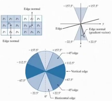
Non-maximal suppression involves thinning the gradient magnitude near edges. We assume \(G_n(x,y)\) as the result of thinning the gradient image. The process follows these steps:
- Find the direction closest to the gradient at location \((x,y)\)
- Identify two neighboring pixels that align with the gradient orientation
- Compare magnitudes: if the magnitude at \((x,y)\) is less than either neighbor in that direction, suppress it (set to zero); otherwise, preserve the original value
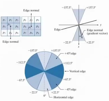
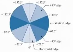
Let’s consider a practical example where we’re working with pixel \(p_5\) and we find the gradient direction to be diagonal. In this case, \(p_3\) and \(p_7\) become the two neighbors of \(p_5\) along that gradient direction. We compare the magnitude of \(p_5\) with both the magnitude of \(p_3\) and \(p_7\). If the magnitude is greater than both neighboring pixels, we retain the value. However, if it’s smaller than the magnitude of either of these two pixels, we suppress that pixel by setting it to zero.
🔴 Why Non-Maximal Suppression Alone Isn’t Enough
Important limitation: While non-maximal suppression effectively thins the edges and helps reduce the number of pixels with low gradient, this step alone is not sufficient for robust edge detection. Additional refinement is necessary through double thresholding and connectivity analysis to remove weak edges even further, ensuring that only the most significant and well-connected edges remain in the final result.
Double Thresholding Implementation
Strong and Weak Edge Separation
The final step involves implementing double thresholding to distinguish between strong and weak edges. We define two threshold values: \(T_H\) (high threshold) and \(T_L\) (low threshold).
$$g_{NH}(x,y) = (g_N(x,y) \geq T_H)$$
$$g_{NL}(x,y) = (g_N(x,y) \geq T_L)$$
$$\Rightarrow g_{NL}(x,y) = g_{NL}(x,y) – g_{NH}(x,y)$$
Since \(T_H\) is greater than \(T_L\), all pixels with value one in \(g_{NH}\) will also be included in \(g_{NL}\). To create a clear separation, we update \(g_{NL}\) by subtracting all the values that are common between the two maps. This ensures that \(g_{NH}(x,y)\) contains only strong edges, while the updated \(g_{NL}(x,y)\) contains only weak edges.
💡 Connectivity Analysis Procedure
- Locate the next unvisited edge pixel \(p\) in \(g_{NH}(x,y)\) and mark it as a valid edge pixel
- Mark as valid edge pixels all the weak pixels in \(g_{NL}(x,y)\) that are connected to \(p\) using eight-point connectivity
- If all non-zero pixels in \(g_{NH}(x,y)\) have been visited, proceed to the final step; otherwise, return to step one
- Set to zero all pixels in \(g_{NL}(x,y)\) that were not marked as valid edge pixels
This process ensures that weak edges are only preserved if they’re connected to strong edges, effectively filtering out noise while maintaining edge continuity.
When comparing the results of regular edge detection versus Canny edge detection, the differences are quite striking. Using image gradient magnitude alone produces edges of varying thickness depending on the strength and shape of the edge – some regions have very thick edges while others have no edges at all. However, when we apply the complete Canny edge detector with all its procedures, we get a much better representation of the edges with consistent, thin boundaries.
Practical Applications
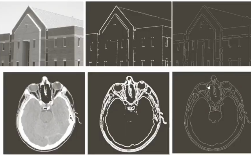
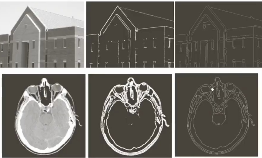
When working with the Canny edge detector, it’s important to understand that the basic output doesn’t provide information about the magnitude or direction of the detected edges. This limitation means that while we can identify where edges exist in an image, we lose crucial details about their characteristics that might be needed for more sophisticated image analysis tasks. However, the Canny edge detector does incorporate an edge linking process as part of its algorithm, which helps connect fragmented edge pixels into continuous contours, creating more coherent and useful edge maps.
7. Edge Linking Strategies
Why Edge Linking Is Essential
The result of edge detection is typically affected by noise and breaks in the edges that are caused by non-uniform illumination and other effects. Edge linking helps create more continuous and reliable edge maps by connecting fragmented edge segments.
Local Edge Linking
In local edge linking, the gap between two edge points is filled if they have similar gradient magnitude and direction. This approach works by examining pixels in each other’s neighborhood – if they share similar gradient characteristics, we connect them together; otherwise, we don’t connect them.
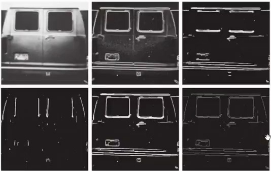
As you can see in the example, we start with the image of the back of a vehicle. In the middle, we have the gradient magnitude, and to the right, we have horizontally connected edge pixels – all the pixels that belong to edges that are horizontal are now connected together. Below that, we have all the vertical edge pixels connected together. Finally, we take the logical OR of these two results and can use morphological techniques for thinning the edges, similar to the non-maximum suppression we saw with the Canny edge detector.
🔴 Limitation of Local Methods
Critical drawback: Local edge linking has a significant limitation – we need to know some information about the edges beforehand. For example, in the vehicle case, we knew that we wanted to connect all the horizontal edges together or all the vertical edges together. But that’s not something we can always know in advance. This limitation naturally leads us to consider more general approaches that don’t require prior knowledge about edge orientation.
Global Edge Linking with Hough Transform
The Power of Parameter Space
The Hough Transform provides an elegant solution to a fundamental problem: how do we identify and connect edge points that belong to the same geometric structure, particularly straight lines? The beauty of the Hough Transform lies in its ability to transform the problem from image space to parameter space, where patterns become much more apparent and easier to detect.
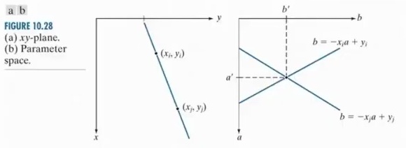
Consider a straight line: \(y=ax+b\). The parameters \((a,b)\) form a parameter space.
💡 The Duality Principle
The core insight of the Hough Transform is the duality between image space and parameter space:
- Edge Point in Image Space: Corresponds to an entire line in parameter space, representing all possible lines that could pass through that point
- Edge Segment in Image Space: With information about both position and orientation, corresponds to a single point in parameter space
This relationship creates a powerful voting mechanism where edge information accumulates in parameter space. When we add up all these contributions from individual edge points and segments, we get distinct peaks in the parameter space. Each peak corresponds to a line in the original image space. The stronger the peak, the more edge points support that particular line hypothesis.
This voting scheme makes the Hough Transform remarkably robust to noise and gaps in edge detection, as it can identify global linear structures even when local edge information is incomplete or corrupted. The method doesn’t require prior knowledge about edge orientation, making it a truly general approach for connecting edge segments that belong to the same geometric structure.
Key Takeaways
- Mathematical Foundation: Image segmentation relies on understanding how first and second-order derivatives behave at different types of intensity transitions – from constant regions to sharp edges
- Point and Line Detection: The Laplacian operator provides a powerful tool for detecting isolated points and lines by measuring how pixels differ from their neighbors, with directional kernels enabling orientation-specific detection
- Edge Detection Methods: While basic gradient-based methods are useful, the Canny edge detector represents the gold standard by combining Gaussian smoothing, gradient computation, non-maximal suppression, and double thresholding to produce optimal edge maps
- Edge Linking Strategies: Local methods work well when edge orientation is known, but the Hough Transform provides a robust global approach that can identify linear structures even in the presence of noise and gaps
- Practical Considerations: Noise sensitivity increases with derivative order, making preprocessing crucial for robust edge detection. The choice between different methods depends on your specific application requirements – whether you need edge magnitude and direction information or just precise edge locations