*Exploring why image classification remains challenging for machines despite being intuitive for humans*

—

## Introduction: Image Classification as a Core Computer Vision Task

Image Classification is a core computer vision task, as shown in the slide title. The task involves taking an input image and assigning it to one of several predefined category labels. When presented with the gray tabby cat image, the system correctly assigns it to the ‘cat’ category.

So when we talk about image classification, we typically have some fixed set of category labels in mind that the algorithm is aware of. In this example, the system must choose from five specific categories: cat, bird, deer, dog, and truck. You just immediately know that this is a cat when you look at the image. But for the computer, that’s not so easy.

While humans can instantly recognize this as a cat, computers face significant challenges in bridging the semantic gap. And the main challenge in image recognition and image classification when we try to do it on machines is this problem we call the semantic gap.

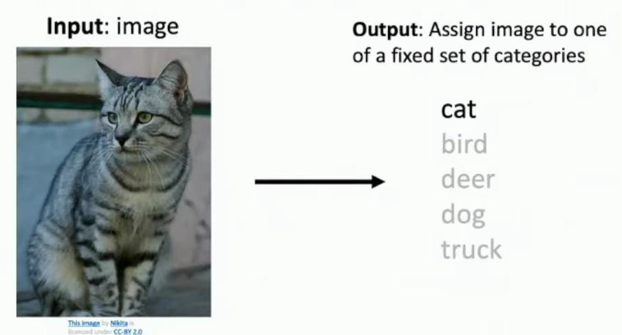
Diagram showing input image of cat and output categories

## Problem: Semantic Gap

When looking at this image of a gray tabby cat, we immediately recognize it as a cat. These perceptions occur when photons hit our retina and undergo complex brain processing. We’re not consciously aware of this processing when viewing images.

However, computers see images as a large grid of numbers between 0 and 255, as shown in the numerical matrix. For this specific image, the computer processes an 800 x 600 x 3 grid, representing the RGB channels. Each pixel contains three values between 0 and 255, representing its color information.

So the problem is that if you look at these grid of numbers, it’s really not obvious at all that this grid of numbers should represent a cat. And there’s no obvious way to convert this grid of raw pixel values into this semantically meaningful category label of cat. And what’s even worse is that this entire grid of numbers can change drastically as we make relatively unassuming changes to the image.

So for example, if we were to imagine changing the viewpoint of this image, maybe if we were to take an image of a photograph of this exact same cat from just a slightly different angle, then to all of us, we would probably recognize it definitely would still recognize it as a cat for sure.

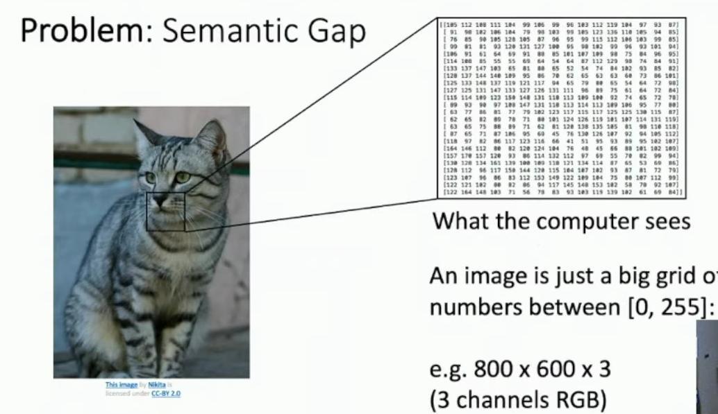
Photo of gray tabby cat

## Challenges: Intraclass Variation

Looking at this group of kittens, we can see how different cats within the same category exhibit significant visual variations – from orange tabbies to gray striped patterns – each producing distinct pixel values when captured by a camera.

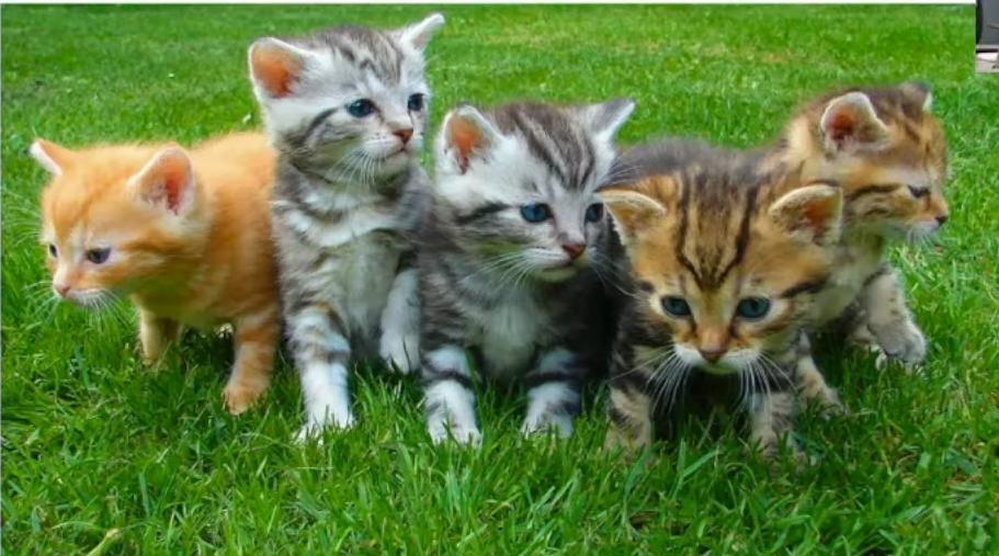
Five kittens of different colors and patterns on grass

## Challenges: Fine-Grained Categories

When recognizing different categories that appear visually similar, like distinct cat breeds, we face significant challenges in fine-grained classification. For example, we might need to distinguish between specific cat breeds like Maine Coon, Ragdoll, and American Shorthair.

These categories present a significant practical challenge in computer vision, as the subtle visual differences between breeds make it difficult to develop algorithms that can reliably distinguish between similar-looking categories based on pixel-level variations.

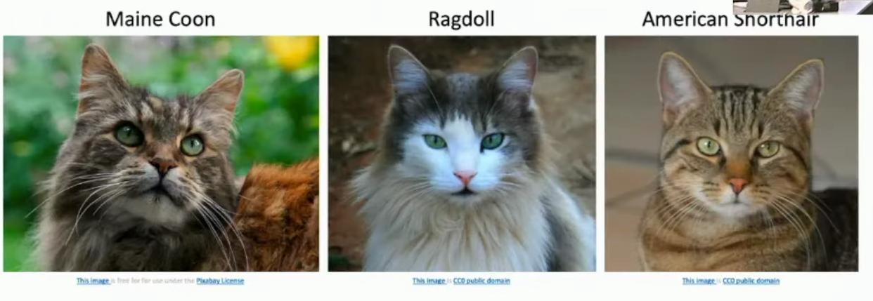
Three cat breed examples: Maine Coon, Ragdoll, and American Shorthair

## Challenges: Background Clutter

Objects we want to recognize can blend into their surroundings through natural camouflage, as shown in both images where the cats’ fur patterns match their environments – one with autumn foliage and another against winter snow.

Our classifiers must be robust to illumination changes, whether capturing images in dark or daylight conditions, as illustrated by the contrast between the bright autumn scene and the muted winter setting.

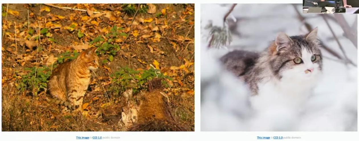
Two cat photos: one in autumn leaves, one in snowy background

## Challenges: Illumination Changes

The underlying semantics of cats remain constant despite dramatic changes in illumination, as demonstrated by the four cat photographs showing the same subject under different lighting conditions. Our algorithms must be robust enough to handle these massive changes in lighting conditions, from deep shadows to bright backlighting, as illustrated in the comparative cat images.

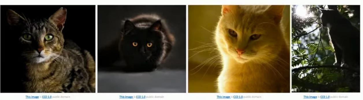
Four cat photos showing same subject in different lighting conditions: tabby in shadow, black cat in dark, white/cream cat in warm light, silhouetted cat in daylight

## Challenges: Deformation

Our algorithms need to deal with deformation, as shown in the title challenge. Cats are particularly deformable objects, as demonstrated by these four images showing cats in various poses – from lounging on their backs to sitting upright.

Sometimes the object that we want to recognize in the image might not be visible hardly at all.

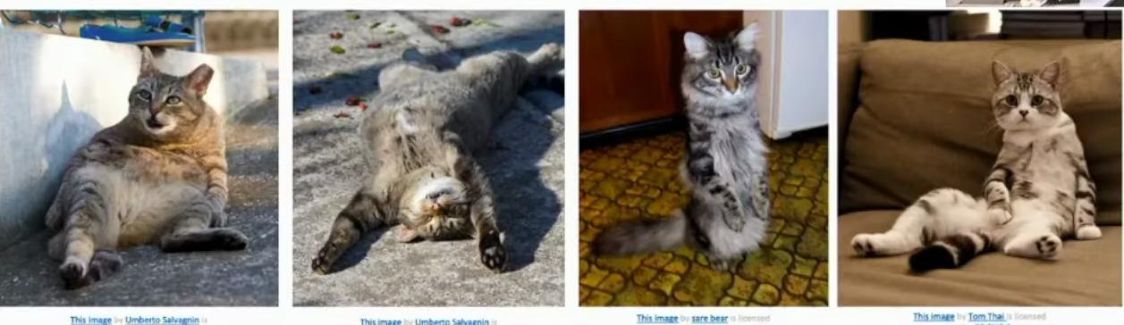
Four photos of cats in different poses and positions

## Challenges: Occlusion

Now you probably intuitively thought that was a cat, as shown in these examples where cats are partially hidden – one under fabric, another in tall grass, and just a tail visible on a couch – demonstrating how we can recognize cats even when partially occluded.

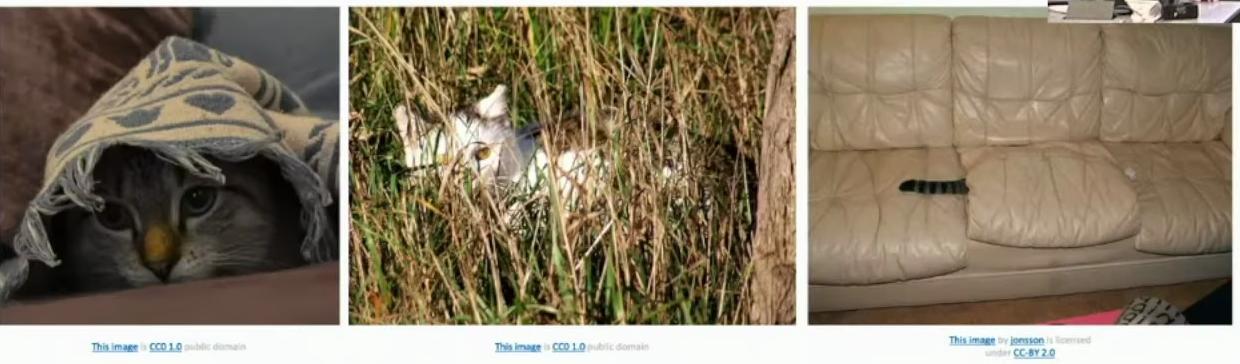
Three images showing cats in various states of occlusion: under fabric, in grass, tail on couch

## The Practical Applications of Image Classification

So we could use image classification for things like medical imaging, medical diagnosis. Maybe we could take pictures of skin lesions and diagnose them as malignant or non-malignant tumors. Maybe we could take pictures of x-rays and try to classify what types of problems could exist in medical images.

This robust image classification could be useful for astronomers who want to go out and collect visual data from telescopes and other types of sensors and then classify what types of phenomenon are out there in the sky. These could also be useful for many other scientific applications like maybe recognizing whales or categorizing many different types of animals that could appear in sensors.

So image classification on its own is this really, really useful problem. And if we could solve it, it can unlock a lot of really powerful and useful applications.

## Image Classification: Building Block for Other Tasks

But what I think is possibly even more interesting and maybe less intuitive is that image classification is also a fundamental building block of different algorithms we might want to perform inside computer vision. Image classification serves as a fundamental building block for other computer vision tasks.

In object detection, the system identifies both the presence and location of objects by drawing bounding boxes around them, as demonstrated with the ‘Person’ and ‘Horse’ labels in the beach scene.

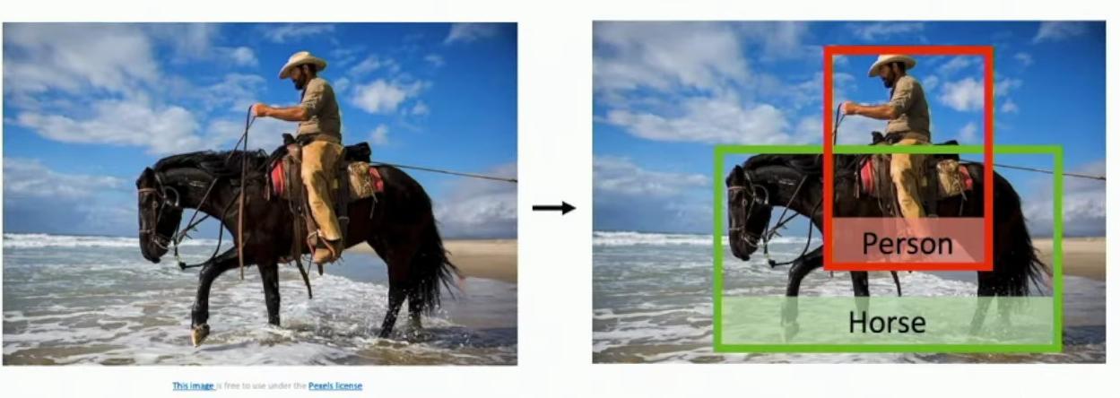
Before/after comparison showing object detection boxes on beach scene with horse and rider

Image classification functions as a foundational component that enables more sophisticated applications like object detection. One approach to object detection involves applying image classification to different sliding windows within the image.

So one way to perform object detection is to just classify different sub regions of the image. So we could look at a sub region over here and then classify it as background horse person car.

## Machine Learning: Data-Driven Approach

So here’s where we come to machine learning. So the idea is that rather than trying to explicitly encode our own human knowledge about what different types of objects look like, instead we’re going to take a data driven approach and have algorithms that can learn from data how to recognize different types of objects in images.

So the basic pipeline for this machine learning system that we’re going to build is that first we want to collect a large data set of images and label them with the types of labels we want our algorithm to predict. So maybe if we want to build a cat versus dog detector, we need to go out and collect a lot of images of cats and dogs and hot dogs and not hot dogs and then class and then and then go and collect human labels for which images are cats and dogs and hot dogs and whatnot.

And then once we collect this large data set, we’re going to deploy some kind of machine learning algorithm which will try to learn statistical dependencies between the input images and the data set and the output labels that we wrote down during the data collection process.

So then once we’ve used our machine learning algorithm to extract these statistical dependencies, we can then evaluate this classifier on new images. One is this, we need to write one function called train which is going to input now a collection of images and they’re associated labels.

## Image Classification Datasets: MNIST

The MNIST dataset consists of 10 classes, representing digits 0 to 9. The images are 28×28 pixels in grayscale format. The dataset provides 50,000 training images and 10,000 test images.

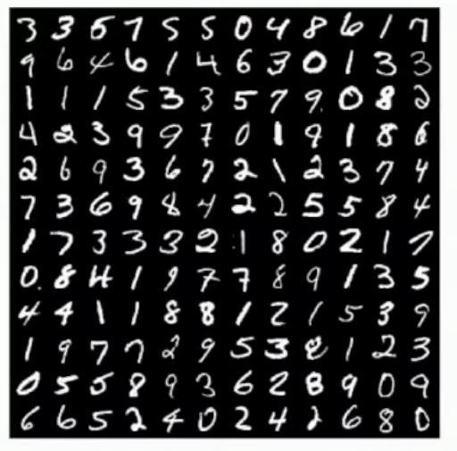
Grid of handwritten digit samples

Looking at the sample images, we can see various handwritten digits displayed in white on black backgrounds, demonstrating the real-world variation in handwriting styles.

The MNIST dataset was developed and deployed for commercial applications, specifically for reading handwritten digits on checks. While MNIST might appear simple, it has a rich history in the development of machine learning algorithms.

But that said, the M-ness data set has sometimes been called the Drosophila of computer vision. So you know that biologists often will go and perform a lot of initial experiments on fruit flies and then they then work up to more interesting animals as they make their discoveries. And this is really similar to the way the lot of practitioners work on M-ness.

## The Limitations and Evolution of Benchmark Datasets

You have to be careful when reading papers that only show results on MNIST, because it’s very common that most algorithms work well on this basic dataset of 28×28 grayscale digit images. Any reasonable machine learning algorithm will get very high performance on MNIST, which includes 50,000 training images and 10,000 test images.

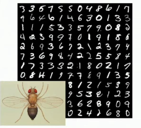
Grid of handwritten digits in black and white

MNIST is treated as the ‘Drosophila of computer vision’ – a proof of concept – but just getting something to work here isn’t enough to impress people anymore, as results often don’t hold on more complex datasets.

## Image Classification Datasets: CIFAR10

So instead, another dataset that you’ll see very commonly used is CIFAR-10. The CIFAR10 dataset consists of 32×32 RGB color images, as specified in the dataset specifications. The dataset contains 10 distinct categories of real-world objects and animals, representing a significant advancement from simple handwritten digits.

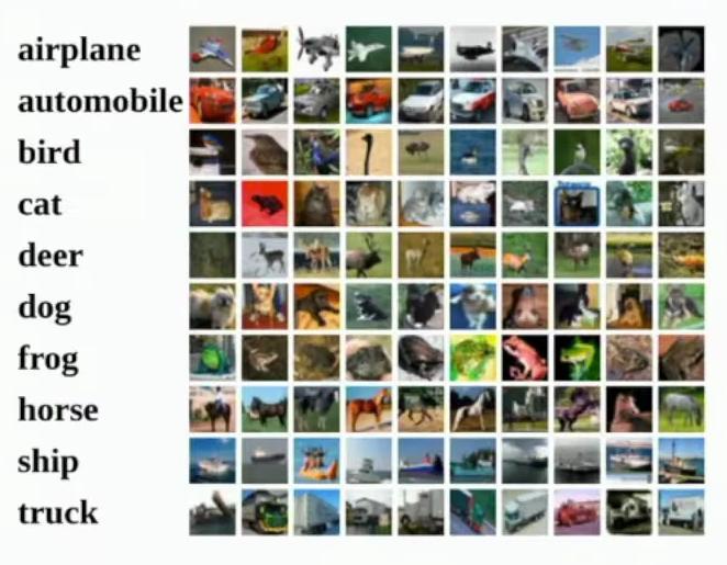
Grid of example images for each category

The categories include airplane, automobile, bird, cat, deer, dog, frog, horse, ship, and truck, each represented by multiple example images. The dataset comprises 50,000 training images (5,000 per class) and 10,000 testing images (1,000 per class).

## Image Classification Datasets: ImageNet

ImageNet has become the gold standard for image classification datasets, containing 1000 distinct classes. When submitting research papers proposing new image classification algorithms, showing results on ImageNet is essentially mandatory to avoid rejection by reviewers.

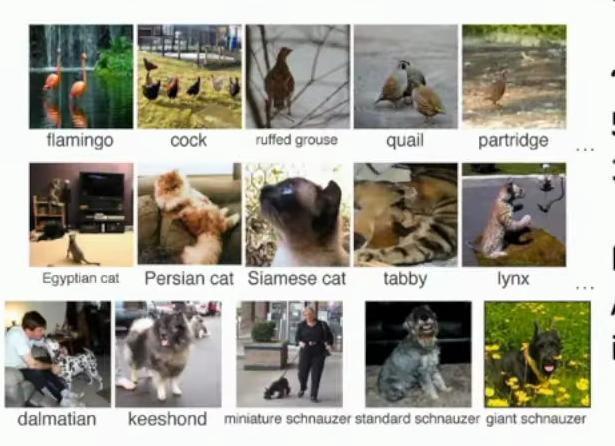
Grid of example images showing different classes like birds and cats

ImageNet contains 1.3M training images (~1.3K per class), 50K validation images (50 per class), and 100K test images (100 per class). The dataset uses Top 5 accuracy as its performance metric, where the algorithm predicts 5 labels for each image and one needs to be correct.

The dataset includes diverse categories ranging from birds like flamingos and quails to various cat breeds such as Egyptian, Persian, and Siamese cats, as well as different dog breeds including schnauzers and dalmatians. And it gives us standard validation and test sets.

## Classification Datasets: Number of Training Pixels

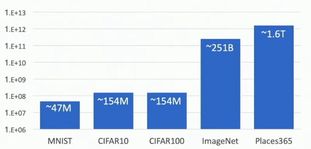
This graph compares the number of training pixels across major classification datasets, ranging from MNIST to Places365. The graph uses a logarithmic scale on the y-axis, ranging from 1.E+06 to 1.E+13.

Bar chart showing pixel counts for different datasets

CIFAR10 and CIFAR100 both contain approximately 154M pixels, about three times more than MNIST’s 47M pixels. ImageNet contains approximately 251B pixels, roughly three orders of magnitude larger than CIFAR datasets. Places365 represents the largest dataset with approximately 1.6T pixels, about six times larger than ImageNet.

And then Places is yet another order of magnitude bigger than ImageNet. So this kind of drives home the point about why ImageNet is somehow a qualitatively different data set than these other ones that you’ll see people work on sometimes.

So that makes results on ImageNet much more convincing, but unfortunately very computationally expensive to work with sometimes. So as a result, we’re kind of sticking with CFR as kind of a sweet middle ground in this course that kind of splits the difference between the complexities of the visual recognition task that show up on ImageNet and the computational affordability of smaller data sets like MNIST.

So what’s also interesting to see from this chart is this increasing trend of data sets getting bigger and bigger and bigger over time. How can we use ever bigger and bigger data sets to enhance the abilities of our algorithms to perform robust classification?

But people have also started thinking in the other direction as well. So one interesting data set to be aware of there is the Omniglott data set.

## Image Classification Datasets: Omniglot

The Omniglot dataset pushes the boundaries of few-shot learning by testing algorithms’ ability to learn from minimal data. Omniglot contains 1,623 different categories of characters. Each category represents a character from various alphabets, as shown in the visual grid of diverse writing systems.

Grid of character examples from different alphabets

The dataset includes characters from 50 different alphabets across various writing systems. Omniglot provides exactly 20 images per category, deliberately limiting the examples to test few-shot learning capabilities.

The challenge is to develop algorithms that can learn effectively from these limited examples per character category. This few-shot classification problem represents a significant area of ongoing research.

## Nearest Neighbor Classification: Our First Learning Algorithm

So basically, we need to write down some kind of distance metric, which can input a pair of images and then spit out some number representing how semantically similar are those two pairs of images in order to perform this nearest neighbor classification.

So one very common choice of this distance metric is a very simple one, just use the L one or Manhattan distance between the pixels of the images. So here what we’re going to do is take our test image. Here we’re imagining a very simple four by four test image that we’ve written down the values of all of its pixels explicitly.

And to compare it to a training image, we simply simply take the absolute value of the differences between all the corresponding pixels in the two images. And then sum up all of these absolute values of all the differences in the corresponding pixels. And that gives us a single number representing the different the distance or difference between those two images.

So one thing to point out here is that you know, if we’ve this kind of satisfies all the normal rules from metric from from from mathematics, right. So if we’ve got two images that are exactly the same, we’ll have a distance of zero things like the triangle inequality are satisfied. This is a reasonably well mathematically defined metric.

So now basically with these couple bits of information, we that’s enough to implement your first learning algorithm. And indeed the nearest neighbor class.

—

## Conclusion: From Challenges to Solutions

We’ve explored the fundamental challenges that make computer vision so difficult for machines – from the semantic gap between raw pixels and meaningful labels, to the myriad variations in viewpoint, lighting, occlusion, and deformation that humans handle effortlessly but confound algorithms.

The journey from traditional hand-coded approaches to machine learning represents a paradigm shift. Rather than explicitly encoding human knowledge about visual features, we now collect large datasets and let algorithms learn statistical patterns from data. We’ve seen how benchmark datasets evolved from simple MNIST digits to complex ImageNet categories, and how the scale of training data has grown exponentially – from millions to trillions of pixels.

With the introduction of distance metrics and nearest neighbor classification, we’ve taken our first steps into practical machine learning for computer vision. While simple, these foundational concepts provide the building blocks for more sophisticated algorithms that can tackle the complex challenges of visual recognition in the real world.

**Part 2 will continue with advanced techniques and deeper learning algorithms…**