# 019 Siamese Network in PyTorch with application to face similarity

Highlights: Hello and welcome back. In today’s post, we’ll discuss and learn a very interesting neural network architecture. We will discuss Siamese Neural Networks, whose goal is to calculate a similarity between two given images. For example, it should tell us how similar two faces are.
Siamese networks were first introduced in the early 1990s by Bromley and LeCun[1] to solve signature verification as an image matching problem It is a very popular solution when it comes to calculating similarities between images. So, let’s start!
Tutorial Overview:
1. What are Siamese Neural Networks ?
Many times, we want to see how similar two pictures are. Moreover, we are interested to see how two faces are similar. One solution that was developed to solve this problem is in fact Siamese Neural Networks. The main idea is that we can use this neural network to distinguish between different faces, cars, and so on.
Let’s look at this example. Imagine we wanted to create an app that would unlock your phone with a photo of your face. To do that we would need to take different pictures and train a model. But, for that model to detect and recognize your face, ideally, we would need a lot of images with different illumination conditions, different head positions, and angles.

Next time we show our face on the camera, it will solve a classification problem and it will check whether we can access the phone or not.

This is a good example where we can train a classification model. We have one person that we are trying to classify and let him use the phone, and, we do not let anyone else access the phone.
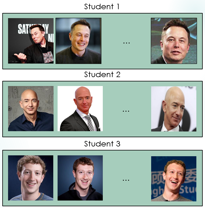
But, now imagine that there is a University that uses a face recognition system so students can enter the exam room without the need for an ID check. For the classification to work, we need multiple images of each student, for example, 10.000 images per student, and we train a classifier.
We can solve this as a classification problem, but what is the problem here?
Well, scalability. Let me explain. If a new student registered for the course, the whole model needs to be retrained. The question now is, can we train only one model and use it for the purpose of face recognition?
The answer is yes, instead of representing the problem as a classification problem, we will represent it as a similarity learning problem. If we would compare two images of the same person, we would get a high similarity score, but on the other hand, if we compare two images of different persons, we get a low similarity score. So, here we are not training our model to classify people, but rather to output a value that indicates the similarity between two images.
It all sounds nice, but how do we actually train our neural network to learn similarities?
Well, the answer is Siamese Neural Networks.
Looking at the image below, we have two inputs, images \(x^{(1)}\) and \(x^{(2)}\), and we pass them through the standard Convolutional Layers, Max Pooling, and Fully connected layers, that you can find in any neural network, to get feature vectors. These feature vectors will later be used as input to determine how similar two images are.
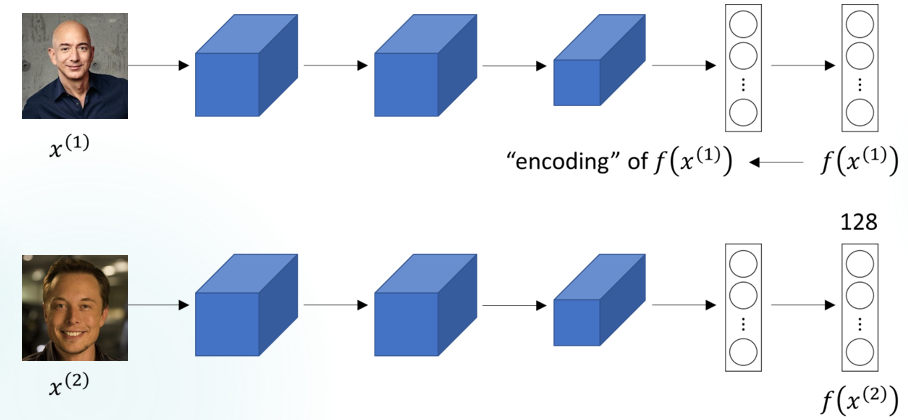
To make classifications, this feature vector is fed into a softmax function, so it is essentially just an encoding of the images. But in this example, where we want to find out if two images are similar, we will not pass it into a softmax function but rather compare these two vectors.
How do we know if two images are of the same person by only comparing two vectors?
Well, these two vectors if they are of the same person, but for example, just a different head pose, should be pretty much similar. On the other hand, if they are of different people these two vectors should be different.
One interesting thing with Siamese Neural Networks is that they are using two identical neural networks at the same time to output the two feature vectors.
In the next step, after we acquire the two vectors, we want to calculate how different the two vectors are. Because of that, a new metric is used, \(d\), L2 norm, which shows us the euclidean distance between the two vectors.
Now, to train our neural network, we need to modify it in such a way that the encoding that it outputs results in a function \(d\). This will tell us how similar two images are.
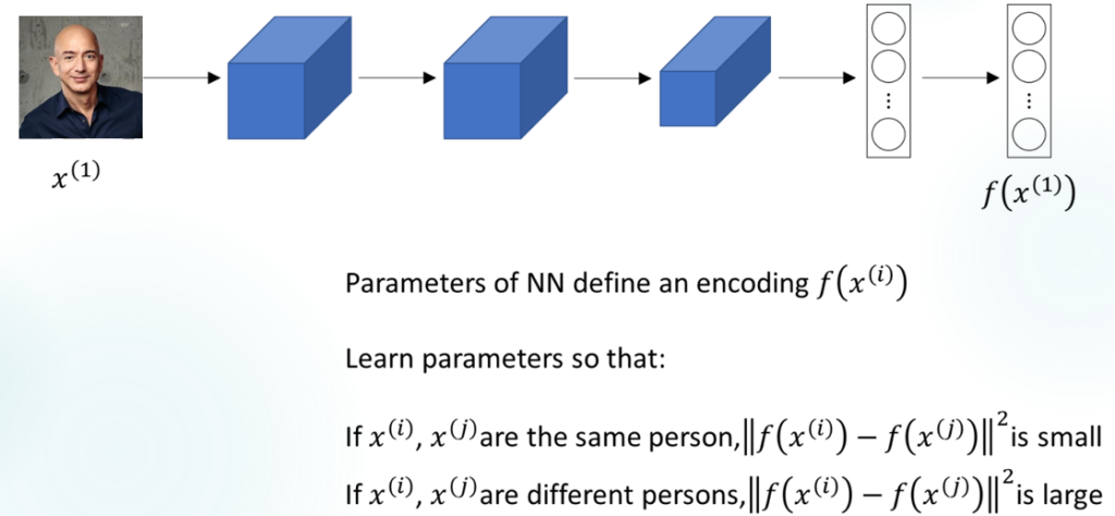
The parameters of a neural network define an encoding \(f(x^{(i)})\), or simply said feature vector. This simply means that given any image \(x^{(i)}\) the network will output a 128 elements long feature vector. We want to learn these parameters, so that when two images are of the same person, \(x^{(i)}\) and \(x^{(j)}\), the distance between the encoding should be small. In contrast, the distance should be large
2. Contrastive Loss Function
How do we calculate the distance or the dissimilarity between these two vectors?
Let’s look at an example when both \(x^{(i)}\) and \(x^{(j)}\) are of the same person, I will denote these two images as \(A\) and \(B\). In this case, we want \(d\) to be a small value:
\(d(A, B) = ||f(A) – f(B)||^2\)
But, what happens when \(x^{(i)}\) and \(x^{(j)}\) are of different people, or a negative pair? Then the distance \(d\) should be large. In such a case, we will not apply the l2 distance norm, or distance function directly, but rather a hinge loss. Why is that?
Well, we want to separate \(f(x^{(i)})\) and \(f(x^{(j)})\) if they are of different people, but we want to separate them until we hit a certain margin \(m\). The idea behind this, is that we don’t actually want to push \(f(x^{(i)})\) and \(f(x^{(j)})\) further and further apart if they are already far from the margin \(m\).
\(d(A, B) = max(0, m^2 – ||f(A) – f(B)||^2)\)
Now, we combine the two together and end up with a formula that is called the Contrastive Loss Function.
This function will calculate the similarity between the two vectors. As we mentioned earlier, the objective of the Siamese networks is not to classify, but rather to differentiate between the images. So a loss function like Cross-Entropy loss is not suitable for this problem.
The Contrastive Loss function evaluates how well the network distinguishes a given pair of images. The function is defined as follows:
\(L(A, B, Y) = (Y)*||f(A) – f(B)||^2 + (1-Y)*\{ max(0, m^2 – ||f(A) – f(B)||^2)\}\)
Looking at the equation at the top, \(Y\) here indicates the label. The label will be 1 if the two images are of the same person, and 0 if the images are of different persons.
The equation has two parts. One positive part, when the two images are of the same people, and one negative part, when the two images are of different people.
From left to right, the first part of the formula is the positive pair, we know when the two images are of the same person, our \(Y\) will be 1. We want to minimize the distance between these two embeddings when the two images are of the same person. So the first part of the equation will be used, but the second part will be ignored because \((1-Y)\) will equal to \(0\).
When we actually have a negative pair, \(Y\) is equal to 0, the left part is ignored and the second part is used. Here we apply the hinge loss, because of the reason mentioned above, and we separate our embeddings further and further away until we hit the margin \(M\).
The output of this equation will be the value that will indicate if the two images are of the same person or not, the same category or not.
This loss function is so to say, the most basic function for learning similarity. Still, even being the most basic, it can solve most of the similarity problems. We will use this function in this tutorial, but if you are asking can we do better?
Yes, yes we can. We could be using the Triplet Loss. The main difference between the Contrastive Loss function and Triplet Loss is that triplet loss accepts a set of tree images as input instead of two images, as the name suggests. This way, the triplet loss will not just help our model learn the similarities, but also help it learn a ranking. What do we mean by ranking?
So, it is not just about similarity, being similar or not, but also about how closer is one image, compared to another. If you want to learn more about Triplet Loss, you can visit this post here, but we will move on and use Contrastive Loss for these examples here.
Let’s tie everything together in the coding part below.
3. Siamese Neural Networks in PyTorch
The first thing we need to do is to import the necessary libraries.
%matplotlib inline
import matplotlib.pyplot as plt
import numpy as np
import random
from PIL import Image
import PIL.ImageOps

import torchvision
import torchvision.datasets as datasets
import torchvision.transforms as transforms
from torch.utils.data import DataLoader, Dataset
import torchvision.utils
import torch
from torch.autograd import Variable
import torch.nn as nn
from torch import optim
import torch.nn.functional as F
The dataset that we will be using is the so-called AT&T dataset. It is a gray-scaled dataset with 400 samples. You can easily download it from our GitHub profile or by running the code below.
!wget https://github.com/maticvl/dataHacker/raw/master/DATA/at%26t.zip
!rm -rf data
!unzip "at&t.zip" -d .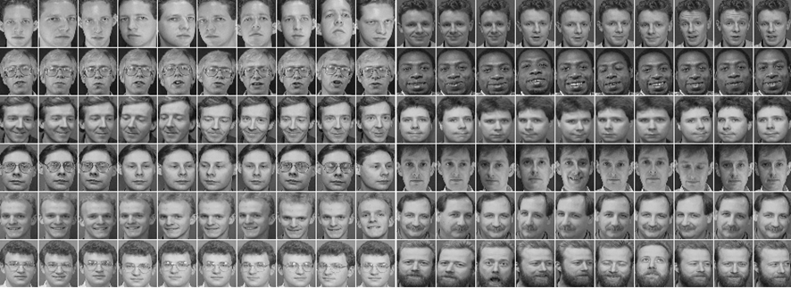
For some easy plotting and visualization, I have created two helper functions as shown in the code block below.
# Showing images
def imshow(img, text=None):
    npimg = img.numpy()
    plt.axis("off")
    if text:
        plt.text(75, 8, text, style='italic',fontweight='bold',
            bbox={'facecolor':'white', 'alpha':0.8, 'pad':10})

    plt.imshow(np.transpose(npimg, (1, 2, 0)))
    plt.show()

# Plotting data
def show_plot(iteration,loss):
    plt.plot(iteration,loss)
    plt.show()
In comparison with the classification neural networks, that take in one image and one label, our Siamese neural network will take as input 2 images and 1 label. To accomplish this, we need to create our own custom Dataset class, SiameseNetworkDataset. It will accept a path where the images are and also the transformations which to apply.
How does this class work?
It will read two images and return them, as well as their label. If they are in the same category, the same person, it will return 0, and otherwise, it will return 1.
class SiameseNetworkDataset(Dataset):
    def __init__(self,imageFolderDataset,transform=None):
        self.imageFolderDataset = imageFolderDataset
        self.transform = transform

    def __getitem__(self,index):
        img0_tuple = random.choice(self.imageFolderDataset.imgs)

        #We need to approximately 50% of images to be in the same class
        should_get_same_class = random.randint(0,1)
        if should_get_same_class:
            while True:
                #Look untill the same class image is found
                img1_tuple = random.choice(self.imageFolderDataset.imgs)
                if img0_tuple[1] == img1_tuple[1]:
                    break
        else:

            while True:
                #Look untill a different class image is found
                img1_tuple = random.choice(self.imageFolderDataset.imgs)
                if img0_tuple[1] != img1_tuple[1]:
                    break

        img0 = Image.open(img0_tuple[0])
        img1 = Image.open(img1_tuple[0])

        img0 = img0.convert("L")
        img1 = img1.convert("L")

        if self.transform is not None:
            img0 = self.transform(img0)
            img1 = self.transform(img1)

        return img0, img1, torch.from_numpy(np.array([int(img1_tuple[1] != img0_tuple[1])], dtype=np.float32))

    def __len__(self):
        return len(self.imageFolderDataset.imgs)
How do we use this custom dataset class?
First, we initialize the dataset by calling the ImageFolder function and passing the path to the training set. We define a simple transformation of only a resize and transformation to tensors. Then, we can call our custom class and pass in the transformation, as well as the folder_dataset we created at the top.
# Load the training dataset
folder_dataset = datasets.ImageFolder(root="./data/faces/training/")

# Resize the images and transform to tensors
transformation = transforms.Compose([transforms.Resize((100,100)),
                                     transforms.ToTensor()
                                    ])

# Initialize the network
siamese_dataset = SiameseNetworkDataset(imageFolderDataset=folder_dataset,
                                        transform=transformation)
For simple visualization purposes let’s look at this example. We create a DataLoader of the siamese_dataset and extract the first batch only. We combine each combination of images, because our siamese_dataset will return two images and one label, and print out the labels.
# Create a simple dataloader just for simple visualization
vis_dataloader = DataLoader(siamese_dataset,
                        shuffle=True,
                        num_workers=2,
                        batch_size=8)

# Extract one batch
example_batch = next(iter(vis_dataloader))

# Example batch is a list containing 2x8 images, indexes 0 and 1, an also the label
# If the label is 1, it means that it is not the same person, label is 0, same person in both images
concatenated = torch.cat((example_batch[0], example_batch[1]),0)

imshow(torchvision.utils.make_grid(concatenated))
print(example_batch[2].numpy().reshape(-1))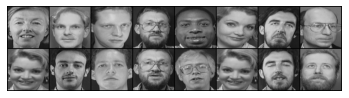
[1. 1. 0. 0. 1. 0. 0. 1.]Looking from left to right, we have our images stacked vertically. The first two images are not of the same person and we have a label of 1. The second two images are also not of the same person, the label is as well 1. But, the 3rd image is of the same person and the label is 0 here, as well as the 4th pair of images.
Now comes the interesting part, training our model. Let’s take a look at the diagram below.
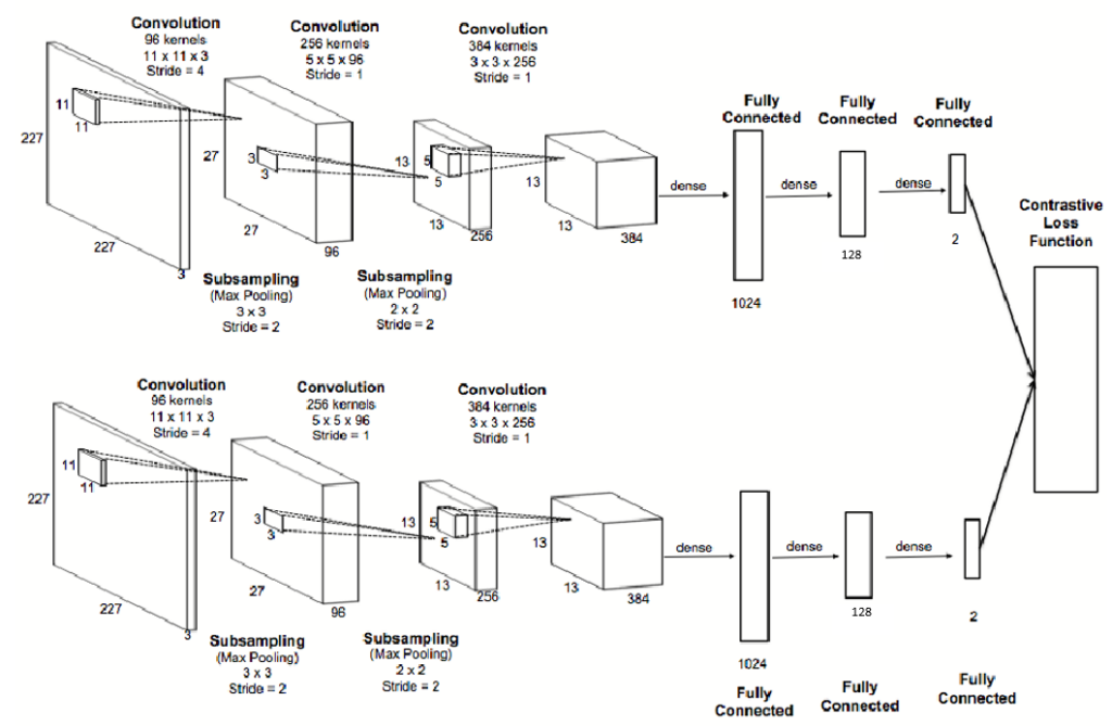
We can see that we have two identical networks, one on top and one below. We pass two images through the two networks and get an output which we pass into the Contrastive Loss Function to calculate the distance or dissimilarity. Now let’s transfer this diagram into PyTorch code.
#create the Siamese Neural Network
class SiameseNetwork(nn.Module):

    def __init__(self):
        super(SiameseNetwork, self).__init__()

        # Setting up the Sequential of CNN Layers
        self.cnn1 = nn.Sequential(
            nn.Conv2d(1, 96, kernel_size=11,stride=4),
            nn.ReLU(inplace=True),
            nn.MaxPool2d(3, stride=2),

            nn.Conv2d(96, 256, kernel_size=5, stride=1),
            nn.ReLU(inplace=True),
            nn.MaxPool2d(2, stride=2),

            nn.Conv2d(256, 384, kernel_size=3,stride=1),
            nn.ReLU(inplace=True)
        )

        # Setting up the Fully Connected Layers
        self.fc1 = nn.Sequential(
            nn.Linear(384, 1024),
            nn.ReLU(inplace=True),

            nn.Linear(1024, 256),
            nn.ReLU(inplace=True),

            nn.Linear(256,2)
        )

    def forward_once(self, x):
        # This function will be called for both images
        # Its output is used to determine the similiarity
        output = self.cnn1(x)
        output = output.view(output.size()[0], -1)
        output = self.fc1(output)
        return output

    def forward(self, input1, input2):
        # In this function we pass in both images and obtain both vectors
        # which are returned
        output1 = self.forward_once(input1)
        output2 = self.forward_once(input2)

        return output1, output2
Our network is called SiameseNetwork and we can see that it looks almost identical to a standard CNN. The only difference that can be noticed is that we have two forward functions ( forward_once and forward ). Why is that?
We mentioned that we pass two images through the same network. This forward_once function, called inside the forward function, will take an image as input and pass it into the network. The output is stored into output1 and the output from the second image is stored into output2, as we can see in the forward function. In this way, we have managed to input two images and get two outputs from our model.
We have seen how the loss function should look like, now let’s code it. We create a class called ContrastiveLoss and similarly as in the model class we will have a forward function. In this forward function we will write our contrastive loss equation from the paragraph before.
# Define the Contrastive Loss Function
class ContrastiveLoss(torch.nn.Module):
    def __init__(self, margin=2.0):
        super(ContrastiveLoss, self).__init__()
        self.margin = margin

    def forward(self, output1, output2, label):
      # Calculate the euclidean distance and calculate the contrastive loss
      euclidean_distance = F.pairwise_distance(output1, output2, keepdim = True)

      loss_contrastive = torch.mean((1-label) * torch.pow(euclidean_distance, 2) +
                                    (label) * torch.pow(torch.clamp(self.margin - euclidean_distance, min=0.0), 2))


      return loss_contrastive
Now that we defined the loss function that we will use, our next step would be definining the data that we will use for the training, and create a data loader object. It will accept our siamese_dataset and also shuffle our data. We will set the num_workers to 8 and also the batch_size to 64.
We will also initialize our model, as well as the loss and optimizer.
# Load the training dataset
train_dataloader = DataLoader(siamese_dataset,
                        shuffle=True,
                        num_workers=8,
                        batch_size=64)

net = SiameseNetwork().cuda()
criterion = ContrastiveLoss()
optimizer = optim.Adam(net.parameters(), lr = 0.0005 )
Following the flow diagram from the top, we can start creating the training loop. We iterate 100 times and extract the two images as well as the label. We zero the gradients and pass our two images into the network, and the network outputs two vectors. The two vectors, and the label, are then fed into the criterion (loss function) that we defined. We backpropagate and optimize. For some visualization purposes and to see how our model is performing on the training set, so we will print the loss every 10 batches.
counter = []
loss_history = []
iteration_number= 0

# Iterate throught the epochs
for epoch in range(100):

    # Iterate over batches
    for i, (img0, img1, label) in enumerate(train_dataloader, 0):

        # Send the images and labels to CUDA
        img0, img1, label = img0.cuda(), img1.cuda(), label.cuda()

        # Zero the gradients
        optimizer.zero_grad()

        # Pass in the two images into the network and obtain two outputs
        output1, output2 = net(img0, img1)

        # Pass the outputs of the networks and label into the loss function
        loss_contrastive = criterion(output1, output2, label)

        # Calculate the backpropagation
        loss_contrastive.backward()

        # Optimize
        optimizer.step()

        # Every 10 batches print out the loss
        if i % 10 == 0 :
            print(f"Epoch number {epoch}\n Current loss {loss_contrastive.item()}\n")
            iteration_number += 10

            counter.append(iteration_number)
            loss_history.append(loss_contrastive.item())

show_plot(counter, loss_history)
Epoch number 0
Current loss 2.2636220455169678
Epoch number 1
Current loss 1.3249046802520752
Epoch number 2
Current loss 1.5688258409500122
...
...
...
Epoch number 97
Current loss 0.00044175234506838024
Epoch number 98
Current loss 0.00035808864049613476
Epoch number 99
Current loss 0.00013359809236135334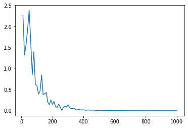
We can now analyze the results. The first thing we can see is that the loss started around 2.2 and ended at a number pretty close to 0.
It would be interesting to see the model in action. Now comes the part where we test our model on images it didn’t see before. As we have done before, we create a Siamese Network Dataset using our custom dataset class, but now we point it to the test folder.
As the next steps, we extract the first image from the first batch and iterate 5 times to extract the 5 images in the next 5 batches because we set that each batch contains one image. Then, combining the two images horizontally, using torch.cat(), we get a pretty clear visualization of which image is compared to which.
We pass in the two images into the model and obtain two vectors, which are then passed into the F.pairwise_distance() function, this will calculate the euclidean distance between the two vectors. Using this distance, we can as a metric of how dissimilar the two faces are.
# Locate the test dataset and load it into the SiameseNetworkDataset
folder_dataset_test = datasets.ImageFolder(root="./data/faces/testing/")
siamese_dataset = SiameseNetworkDataset(imageFolderDataset=folder_dataset_test,
                                        transform=transformation)
test_dataloader = DataLoader(siamese_dataset, num_workers=2, batch_size=1, shuffle=True)

# Grab one image that we are going to test
dataiter = iter(test_dataloader)
x0, _, _ = next(dataiter)

for i in range(5):
    # Iterate over 5 images and test them with the first image (x0)
    _, x1, label2 = next(dataiter)

    # Concatenate the two images together
    concatenated = torch.cat((x0, x1), 0)

    output1, output2 = net(x0.cuda(), x1.cuda())
    euclidean_distance = F.pairwise_distance(output1, output2)
    imshow(torchvision.utils.make_grid(concatenated), f'Dissimilarity: {euclidean_distance.item():.2f}')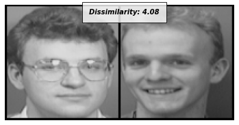
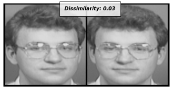
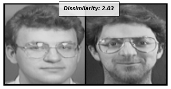
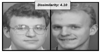
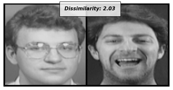
Looking at the results, we can see that the dissimilarity number is pretty close to zero when the two images are of the same person, which is great. The dissimilarity number is large when the two images are of different people, as we hoped!
Summary
In this post, we have explained what Siamese neural networks are and how they work. We have seen that it is not a classification problem, and learned a new loss function, Contrastive Loss Function. In the end, we have implemented our own Siamese Neural Network in PyTorch and trained it in such a way that it can tell us if two images are of the same person, we have made a simple person recognition model!
References:
[1] Bromley and LeCun.“Signature Verification using a “Siamese” Time Delay Neural Network”.