#004B The Computation Graph – Example
The Computation graph – Example
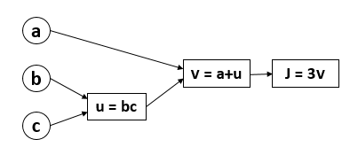
Let’s say that we’re trying to compute a function \(J\), which is a function of three variables \(a\), \(b\), and \(c\) and let’s say that function \(J\) is \(3(a+bc)\).
 |
 |
Computation of this function has actually three distinct steps:
- Compute \( bc \) and store it in the variable \(u\), so \(u = bc \)
- Compute \(v = a + u \),
- Output \(J \) is \(3v\).
Let’s summarize:
$$ J(a, b, c) = 3(a + bc) $$
$$ u = bc $$
\(v = a + u \)
$$ J = 3v $$
As we can see, the computation graph comes handy when there is some distinguished or some special output variable, such as \(J\) in this case, that you want to optimize. And in the case of a logistic regression, \(J\) is of course the cost function that we are trying to minimize.
In this simple example we see that, through a left-to-right pass, you can compute the value of \(J\).
We have learned the way of using the computation graph to compute the function \(J\), and how to figure out derivative calculations of the function \(J\).
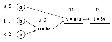
Now we want, using a computation graph, to compute the derivative of \(J\) with respect to \(v\). Let’s get back to our old picture, but with concrete parameters.

We can see from the picture, that we have assigned values to our \(a\), \(b\) and \(c\) parameters and that we are able to compute the output of our system: 33.
First, let’s see the final change of value \(J\) if we change \(v\) value a little bit:
$$ J = 3v $$
\(v = 11 \) \(\rightarrow \) \(11.001 \)
\(J = 33 \) \(\rightarrow \) \(33.003 \)
$$ \frac{33.003 – 33 }{11.001 – 11} = \frac{0.003 }{0.001} = 3 $$
$$ \frac{\mathrm{d} J }{\mathrm{d} v} = 3 $$
We can get the same result if we know calculus:
\(f(a) = 3a \) \(\Rightarrow \) \(\frac{\mathrm{d} f }{\mathrm{d} a} = 3 \)
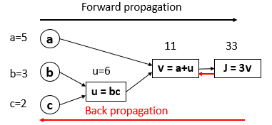
We emphasize that calculation of \(\frac{\mathrm{d} J }{\mathrm{d} v} \) is one step of a back propagation. Next picture depicts forward as well as backward propagation:

Next, what is \(\frac{\mathrm{d} J }{\mathrm{d} a} \)? It’s actually the slope of our function. With this information we may determine if our function is increasing or not. This is very important piece of information: if we know this we are actually able to find global optima of our function (of course under already stated assumptions).
If we increase \(a\) from 5 to 5.001, \(v\) will increase to 11.001 and \(J\) will increase to 33.003. So, the increase to \(J\) is the three times the increase to \(a \) so that means this derivative is equal to 3.
\(a = 5 \) \(\rightarrow \) \(5.001 \)
\(v = 11 \) \(\rightarrow \) \(11.001 \)
\(J = 33 \) \(\rightarrow \) \(33.003 \)
$$ \frac{\mathrm{d} J }{\mathrm{d} a} = \frac{\mathrm{d} J }{\mathrm{d} v} \frac{\mathrm{d} v }{\mathrm{d} a} $$
$$ \frac{\mathrm{d} J }{\mathrm{d} a} = 3 $$
One way to break this down is to say that if we change \(a\), that would change \(v\) and through changing \(v\) that would change \(J\).
By increasing \(a\), how much \(v\) is increased? This is determined by \(\frac{\mathrm{d} v }{\mathrm{d} a} \). The change in \(v\) will cause the value of \(J \) also to increase. This is called a chain rule in calculus:
$$ \frac{\mathrm{d} J }{\mathrm{d} a} = \frac{\mathrm{d} J }{\mathrm{d} v} \frac{\mathrm{d} v }{\mathrm{d} a} $$
$$ \frac{\mathrm{d} J }{\mathrm{d} u} = ? $$
\(u = 6 \) \(\rightarrow \) \(6.001 \)
\(v = 11 \) \(\rightarrow \) \(11.001 \)
\(J = 33 \) \(\rightarrow \) \(33.003 \)
$$ \frac{\mathrm{d} J }{\mathrm{d} u} = \frac{\mathrm{d} J }{\mathrm{d} v} \frac{\mathrm{d} v }{\mathrm{d} u} = 3 \cdot 1 $$
Now, let’s calculate derivative \(\frac{\mathrm{d} J }{\mathrm{d} u} \).
Finally, we have to find the most important values: value of \(\frac{\mathrm{d} J }{\mathrm{d} b} \) and \(\frac{\mathrm{d} J }{\mathrm{d} c} \). Let’s calculate them:
|
$$ \frac{\mathrm{d} J }{\mathrm{d} c} = ? $$ \(c = 2 \) \(\rightarrow \) \(2.001 \) \(u = 6 \) \(\rightarrow \) \(6.003 \) \(J = 33 \) \(\rightarrow \) \(33.009 \) $$ \frac{\mathrm{d} u }{\mathrm{d} c} = \frac{0.003 }{0.001} = 3 $$ $$ \frac{\mathrm{d} J }{\mathrm{d} c} = \frac{\mathrm{d} J }{\mathrm{d} u} \frac{\mathrm{d} u }{\mathrm{d} c} = 3 \cdot 3 = 9$$ |
$$ \frac{\mathrm{d} J }{\mathrm{d} b} = ? $$ \(b = 3 \) \(\rightarrow \) \(3.001 \) \(u = 6 \) \(\rightarrow \) \(6.002 \) \(J = 33 \) \(\rightarrow \) \(33.006 \) $$ \frac{\mathrm{d} u }{\mathrm{d}b} = 2 $$ $$ \frac{\mathrm{d} J }{\mathrm{d} b} = \frac{\mathrm{d} J }{\mathrm{d} u} \frac{\mathrm{d} u }{\mathrm{d} b} = 6 $$ |
In the next post we will learn how to applying gradient descent on m training examples.