GANs #004 Variational Autoencoders – in-depth explained

Highlight: In this post, we will be discussing Variational Autoencoders (VAE). In order to fully understand the underlying ideas, we need to have a basic understanding of traditional Autoencoders. Luckily, we have already written about them in our previous posts. This post will consist of several topics. First, we will review autoencoders. Then, we will give some review of basic probability concepts. Next, we will explain what Kullback Leibler divergence is. In addition, we will talk about the loss function and how it can be derived.

1. Stacked Autoencoders
2. Probability brush-up
3. Kullback-Leibler divergence
4. More insights into VAEs
5. Derivation of the Loss Function
6. Optimization and Reparameterization Trick

1. Stacked Autoencoders

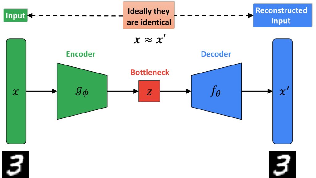
So, the first concept that we’re going to review is autoencoders. Sometimes, we also call them the stacked autoencoders. One application of autoencoders is image compression. The pipeline is commonly presented as a block diagram in the following way.

We have an input image that goes into an encoder part. The input can be a simple image like the one from the MNIST data set. As you can see here, it is a digit \(3\). Once this digit passes through the network, we want to reconstruct the original image at its output as closely as possible. For that, we use the cost function \(L \). Here, we have two parameters \(\theta \) and \(\phi \). This is the equation that we use:

Cost function:

$$ L\left ( \theta ,\phi  \right )= \frac{1}{N}\sum_{i= 1}^{N}\left [ x^{\left ( i \right )}-f_{\theta }\left ( g_{\phi }\left ( x^{(i) } \right ) \right ) \right ]^{2} $$

As usual, it represents a squared pixel by pixel difference, and then, we square the values, apply the summation and divide this value by the number of samples. This is a well-known “Mean Squared Error” cost function (MSE). In general, note that the loss function is defined for a single image, whereas the cost function represents the averaged loss over the complete training dataset. 

So, we can divide an autoencoder architecture in three parts:

1. We have an encoder and that’s usually a neural network. It is specified here with the function \(g_{\phi } \). 
2. Then, we have a bottleneck layer that can be seen as a vector \(z \) that we need to design. Usually, the size of the bottleneck is much smaller than the size of the encoder’s input. 
3. The third part is the decoder that is specified with the function \(f \) and its parameters \(\theta \). The decoder has to reconstruct the replica of the original image from a relatively small number of elements in a vector \(z\).

Commonly, both encoder and decoder parts are neural networks. As you know, the neural network consists of weights and biases. So, if you are wondering what these parameters \(\theta \) and \(\phi \) are, they are actually the weights and biases of a neural network. 

Once again, we see that the cost function is calculated in a way that the original image is subtracted from the reconstructed and pixel-by-pixel difference is squared. All these values are summed, and then, we take an average across all samples that we have used to train our autoencoder. Therefore, our goal is to minimize the cost function by finding optimal parameters \(\theta \) and \(\phi \).

Now, we will have a more detailed look into the second term of the cost function. It is a reconstructed image at the output. So, we have this term reconstructed image and it’s interesting how we derive this term. First, we apply the function \(g_{\phi } \) to the original input image, and then, we apply the decoder function \(f_{\theta } \). So, by applying these two functions we obtain the reconstructed image. In addition, you can see these functions \(g_{\phi } \) and \(f_{\theta } \) are nothing else but two neural nets in the autoencoder.

$$ L\left ( \theta ,\phi  \right )= \frac{1}{N}\sum_{i= 1}^{N}\left [ x^{\left ( i \right )}-f_{\theta }\left ( g_{\phi }\left ( x^{(i) } \right ) \right ) \right ]^{2} $$

By now, you are probably asking:

Why are we using something as an input, and then reconstructing it? We will talk more later, but the idea is that we want to represent image as a vector \(z\). This vector will be of a much smaller dimension. If we succeed to reconstruct back our original input image, we can be happy with our results!

So, where do we use autoencoders? 

One application of the autoencoder architecture is the so-called denoising autoencoder. In this case, we have our input image as before. However, we actually degrade this image by adding noise to it. That’s commonly done by adding a certain type of noise like a Gaussian noise.

So, we do not have the original image as the input, but a noisy version of this image. In denoising autoencoders, everything else is the same as for the traditional autoencoder. We have the encoder, the bottleneck, and the decoder. In addition, our loss function remains the same as well. However, pay attention that now in this formula we have \(\tilde{x} \) and not our original \(x \). This means that our input is a partially destroyed input image (a noisy image).

$$ \tilde{x}^{\left ( i \right )}\sim \chi \left ( \tilde{x}^{\left ( i \right )}\mid x^{\left ( i \right )} \right ) $$

$$ L\left ( \theta ,\phi  \right )= \frac{1}{N}\sum_{i= 1}^{N}\left [ x^{\left ( i \right )}-f_{\theta }\left ( g_{\phi }\left ( \tilde{x}^{\left ( i \right )} \right ) \right ) \right ]^{2} $$

Logically, you can ask yourself the following question: Why are we actually using denoising autoencoders? We have an input image, and then, we obtain some reconstructed image that resembles the noisy version.

So, the idea is that this noise can be seen as some regularization term that also prevents this network from overfitting. On the other hand, this reconstruction is actually learning in such a way that we create a set of small and robust feature vectors \(z \). So, you should be aware that a vector \(z \) is of a much smaller dimension than the original input vector (image size). Commonly, in some dataset, like MNIST, our input consists of \(28\times 28 \) pixels and that equals \(784 \) pixel image. The size of the bottleneck \(z \) in our case can be as low as 10-30. This small number of vector elements we can pass forward through the decoder and reconstruct our original image.

In this way, we have actually compressed our image with a large factor. So, for instance, in the communication applications, we can just send these 10-30 elements and this will significantly reduce the bandwidth of the communication channel. So, the advantage is the large compression ratio that we can obtain with this method.

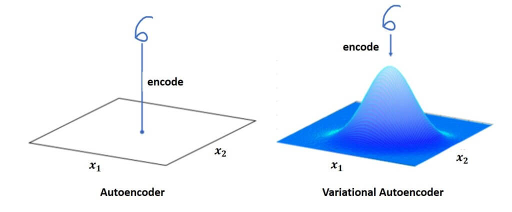
Now, while we are still in the introductory parts, let’s have a look at Variational Autoencoder (VAE) architecture. You can see the difference between traditional autoencoders. Now, we don’t have the classic bottleneck vector.

In contrast, we have a so-called probabilistic encoder where the function \(q_{\phi } \) is now given as a conditional probability.

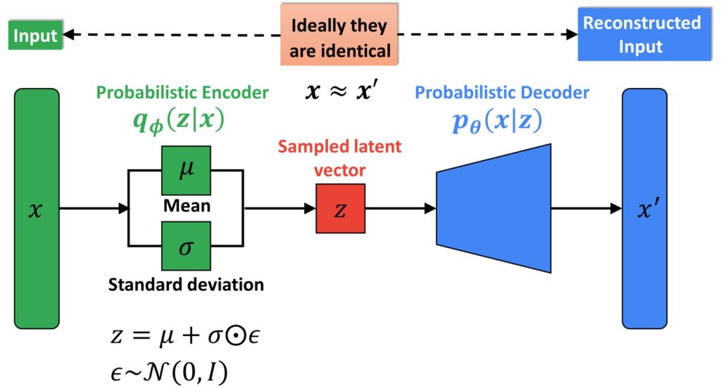
So, instead of the exact values of a vector \(z \), our network needs to learn parameters. These parameters are mean (\(\mu \)) and standard deviation (\(\sigma \)) of the multivariate probabilistic distribution. From here, we obtain a vector \(z \) in such a manner that we actually generate samples from this estimated distribution.

Next, we can see that the cost function of VAE is now defined using the mathematical expectation (E) :

$$ Loss= L\left ( \theta ,\phi  \right )= -E_{z\sim q_{\phi }\left ( z\mid x \right )}\left [ p_{\theta }\left ( x\mid z \right ) \right ]+D_{KL}\left ( q_{\phi }\left ( z\mid x \right )\parallel p_{\theta }\left ( z \right ) \right ) $$

As a result, you can see that the loss function is now quite different, and it consists of two terms. At the moment, we can just say that they are quite complex. Therefore, in order to fully understand them, we will have to go back to probability theory and brush up on our probability skills. Let’s do this!

2. Probability brush-up

So, let’s briefly review the prerequisites of probability theory that we will need for variational autoencoders. It will require us to refresh our knowledge about the following four concepts.

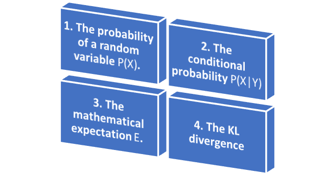
1. We are going to start with the basic concept which is The probability of a random variable \(P\left ( X \right ) \). 
2. Then, we will have a Conditional probability of \(X \) given a random variable \(Y \) (\(P\left ( X|Y \right ) \))
3. Next, we have an operation – Mathematical expectation \(E \). 
4. Finally, we will explain KL Divergence which is more advanced concept. 

The probability of a random variable

So, first, we define \(P\left ( X \right ) \). It is just a probability function of a random variable \(X \). Here, \(X \) is written as a capital letter and it shows what is the probability for a certain discrete event. For instance, \(X \) can be a result of a coin tossing, and then, we have a probability of 50% that it will be heads or tails. 

Conditional probability

On the other hand, we have a conditional probability and now things are becoming a little bit more complex. In this case, we were interested in the probability of an event \(X \) given \(Y \). What does this mean? Well, we already know that \(Y \) has happened and now we are interested in the probability of \(X \). Let’s say that \(X \) is a daily temperature. \(Y \) is a random variable that describes whether there is rain during a certain day. So, now, if there was a rainy day, we have a higher chance that the daily temperature will be lower. This is common for a rainy day. The added information that there was rain changes our perception. That is, the probability of the daily temperature is changed. If it was a rainy day, chances for a lower temperature will be higher with this added insight. That’s an example of conditional probability.

While we speak about conditional probability, we should mention one of the most famous theorem in probability. It is the Bayes’ theorem:

So, we can say that the first term \(P\left ( Y\mid X \right ) \) is a posterior probability, whereas \(P\left ( Y \right ) \) is called a priori probability. Using this well-known theorem, we will be able to solve some challenges in VAE. In addition, we should mention that we have a ratio that is known as a likelihood ratio. It is defined as \(\frac{P\left ( X\mid Y \right )}{P\left ( X \right )} \). 

On the other hand, we have another representation of a conditional distribution \(P\left ( Y\mid X \right ) \) and we can represent it as a joint distribution divided by \(P\left ( X \right ) \) :

$$ \frac{P\left ( X,Y \right )}{P\left ( X \right )} $$

And finally, one very important concept that we need to remind ourselves, of is a theorem of total probability. So, this theorems states as follows:

Let \(Y_{1},Y_{2},Y_{3}…Y_{N} \) be a set of mutually exclusive events.

That means that \(Y_{i}\cap Y_{j}= 0 \) or it is an empty set. In this case, if the event \(X \) is the union of mutually exclusive events then we have a formula:

$$ P\left ( X \right )= \sum_{i= 1}^{N}P\left ( X\mid Y_{i} \right )P\left ( Y_{i} \right ) $$

Also, we should remind ourselves what mutually exclusive means. So, if we draw two circles that represent events, they are mutually exclusive if there is no intersection between those two events. On the other hand, if there is an intersection, they are not mutually exclusive.

Furthermore, another very important concept in probability theory is expectation. The expectation of a random variable \(X \), and we write this as \(E\left ( X \right ) \), states as follows.

It is the expected value of a random variable where the variable is given as a weighted average of the possible values that variable \(X \) can take. Moreover, every variable is weighted according to the probability of that event defined by \(X \).

$$ E\left ( X \right )= \sum_{i= 1}^{K}X_{i}P\left ( X= X_{i} \right ) $$

This is given with the following formula where \(E\left ( X \right ) \) is a sum over all possible events that \(X \) can take. We can see that \(X_{i} \) is the real value of a random variable \(X \) multiplied with the probability that the event \(X_{i} \) happens.

Another thing to note is that the \(E\left ( X \right ) \) can be written as \(E_{P}\left ( X \right ) \). This implies that we have an expectation operator over a random variable \(X \) given the probability \(P \).

Examples

Example 1. The previous concepts are simple to explain if we imagine that we have a die and we toss it. So, a probability to get a number four, is given as \(P\left ( 4 \right )= \frac{1}{6} \). 

So, how have we arrived at this conclusion? Super easy. A die has \(6 \) numbers on it. Once we toss it, each of these 6 numbers will have an equal probability to show. We say that it is a fair die. So, the probability to get the number \(4 \) is actually \(1/6 \).

Example 2. The following example will give us more insight into conditional probability. So, once again we can observe a tossing of a fair die. And initially, we can ask what is the probability that we get a number \(4 \)? We know that \(P\left ( 4 \right )= \frac{1}{6} \).

However, now we can redefine our statement and ask ourselves what is the probability that we get a \(4 \) if we know that the number that we obtained is even. So, now this will be the additional information that we have about our experiment. Someone observed an experiment and told us that it was an even number. Now, we are asked what is the probability that we get a number \(4 \). Obviously, our set of possible events has changed. We cannot get six possible numbers, but only three potential even numbers: \(2, 4\) and \(6 \). Now, our probability to get the number \(4 \) has changed. So, \(P\left ( 4 \right )= \frac{1}{3} \), because we have obtained additional information about this event. That’s an example of conditional probability and how observation of one event affects the probability of the other one.

The following image illustrates another example of conditional probability. It is the famous Monty Hall problem. This probability puzzle is based on the American television game show Let’s Make a Deal and named after its original host, Monty Hall.

Example 3. In addition, we can use the example 2 to illustrate what is the expectation of a random variable \(X \). So, we will write a set of possible outcomes for \(X \). These are the numbers from one to six. And a probability, in case that it is a fair die, is \(1/6 \) for each of them. So, it’s very easy to calculate the expectation:

$$ X= \left \{ 1,2,3,4,5,6 \right \} $$

$$ P\left ( X \right )= \frac{1}{6} $$

$$ E\left ( X \right )= \sum_{i= 1}^{6}X P\left ( X \right )= \frac{1}{6}+\frac{2}{6}+\frac{3}{6}+\frac{4}{6}+\frac{5}{6}+\frac{6}{6}= 3.5 $$

This is easy to calculate and as the final result, we get \(3.5 \).

Ok, so far so good. We have covered a lot and we are now ready for Kullback- Leibler divergence. 

3. Kullback- Leibler divergence

The concept that we are now going to explain is the so-called Kullback-Leibler divergence and it’s commonly referred to as the KL divergence. Basically, this concept can be related to a distance or to a similarity measure. For instance, imagine that we have two points in a 2D space. We can define a distance between them. It tells us how far apart they are. Usually, we use the most common distance and it is the well-known Euclidean distance. The same concept we apply for two geographic locations. We can calculate how far away the two cities are. 

On the other hand, imagine that we want to calculate how much two probability distributions are similar. 

We cannot apply a concept as simple as the Euclidean distance. Therefore, we need to apply something more complex for two probability distributions. Let’s have a look at the following example. The first distribution can be a Gaussian distribution. It is shown in the image on the left. And the second one can be, for instance, a uniform distribution. So, the first one we can denote as \(p\left ( x \right ) \), and the second one we can denote as \(q\left ( x \right ) \).

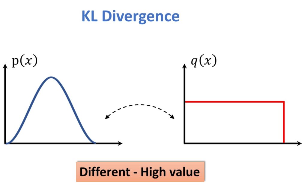
Obviously, we see that these two distributions are very different. For them, if we want to measure their dissimilarity, this number will be relatively high in a sense of a KL divergence measure. 

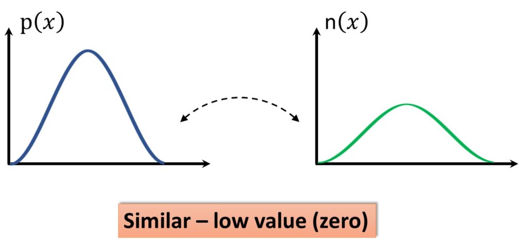
On the other hand, we can have two different distributions that we also want to compare. We can have \(p\left ( x \right ) \) and the second one can be \(n\left ( x \right ) \). We see that they are very similar. There is just a subtle difference between those two distributions and for those two distributions, we would like to get approximately \(0 \) for their similarity measure.

Now, we will introduce a little bit more formal definition of the Kullback-Leibler divergence. 

It is a measure of how one probability distribution differs from the other one. And for this, we will look at discrete probability distributions and calculate KL divergence. So, the KL divergence is given by the following formula:

$$ D_{KL}\left ( P\parallel  Q \right )= \sum_{x}^{ }P\left ( X= x \right )\log \left ( \frac{P\left ( X= x \right )}{Q\left ( X= x \right )} \right ) $$

That’s actually the sum over all possible values of \(X \) and it sums the product terms. Or simplified, it can be written like the second equation that we have here:

$$ D_{KL}\left ( P\parallel  Q \right )= \sum_{x}^{ }P\left ( x \right )\log \left ( \frac{P\left ( x \right )}{Q\left ( x \right )} \right ) $$

At the first sight this can be a little bit too complicated. However, once we go through the simple example, we will see that it actually makes a lot of sense. So, we will define two distributions. They will be the so called discrete distributions because the only value that we can have here are \(0, 1, 2 \). So, \(Q \) is defined as \(0.36 \) for a value 0, \(0.48 \) for 1 and \(0.16 \) for 2. On the other hand, \(P \) is defined as a uniform distribution with the probability of \(1/3 \) and for each of these three events. A simple way to proceed is to apply the KL equation above and we can simply plug in these values.

$$ D_{KL}\left ( P\parallel  Q \right )= \frac{1}{3}\log \left ( \frac{0.333}{0.36} \right )+\frac{1}{3}\log \left ( \frac{0.333}{0.48} \right )+\frac{1}{3}\log \left ( \frac{0.333}{0.16} \right ) = 0.09 $$

So, we have obtained the following terms, and as a result, we will obtain the resulting divergences \(0.09 \). It’s actually quite a small number as we can see.

Therefore, we can infer from this example two properties of KL divergence. The first one is that both KL of P&Q and KL of Q&P will be larger or equal to \(0 \). On the other hand, if we observe the previous example, we can see that there is the scalar that multiplies the logarithmic value, and it is related to the probability we take as the first argument. We see that KL is not commutative or not symmetric operation. Hence, it is very important to accurately specify the order of the two probabilities since the symmetric property does not hold.

Properties:

\(KL\left ( P\parallel Q \right ) \) or \(KL\left ( Q\parallel P \right )\geq 0 \)

$$ KL\left ( P\parallel Q \right ) \neq KL\left ( Q\parallel P \right ) $$ (not symmetric)

KL divergence of two Gaussian disstributions. In VAE, we will see that the Gaussian distribution plays a cruical role. Hence, we want to investigate for two multivariate Normal (Gaussian) distributions is how KL divergence can be derived. First of all, we define a vector \(x \) as a random variable of size \(K \) and we have:

$$ p\left ( x \right )=\mathcal{N} \left ( x; \mu_{1},\Sigma _{1} \right ) $$

a \(q\) is defined in a similar manner:

$$ q\left ( x \right )= \mathcal{N}\left ( x; \mu_{2},\Sigma _{2} \right ) $$

So \(\mu _{1} \) and \(\mu _{2} \)  are the mean values and \(\Sigma _{1} \) and \(\Sigma _{2} \) are the covariance matrices. Let’s first remind ourselves that the formula for the multivariate normal density is defined with the following equation:

$$\mathcal{N} \left ( x;\mu ,\Sigma  \right )= \frac{1}{\sqrt{\left ( 2\pi  \right )^{K}\left | \Sigma \right |}} \exp \left ( -\frac{1}{2}\left ( x-\mu  \right )^{T}\Sigma ^{-1}\left ( x-\mu \right ) \right ) $$

What is interesting here is that we have this term \(\left ( 2\pi \right )^{K} \) meaning that \(X \) is of dimension of \(K \). So, we can write the final result:

$$ D_{KL}\left ( p\left ( x \right )\parallel q\left ( x \right ) \right )= \frac{1}{2}\left [ \log \frac{\left | \Sigma _{2} \right |}{\left | \Sigma _{1} \right |}-d+tr \left ( \Sigma _{2}^{-1} \Sigma _{1}\right ) +\left ( \mu _{2}-\mu _{1} \right )^{T}\Sigma _{2}^{-1}\left ( \mu _{2}-\mu _{1} \right )\right ] $$

It can be puzzling how actually we arrived to this formula, so let’s derive this term step by step.

We will start with several basic definitions that we plug in into KL formula:

\(K L(p(x) \| q(x))=\sum_{x} p(x) \log \left(\frac{p(x)}{q(x)}\right) \)

\(p(x)=\frac{1}{\sqrt{(2 \pi)^{K}}\left|\Sigma_{1}\right|} \exp \left(\frac{-\left(x-\mu_{1}\right)^{\top} \Sigma_{1}^{-1}\left(x-\mu _{1}\right)}{2}\right) \)

\(\log p(x)= -\frac{k}{2} \log (2 \pi)-\frac{1}{2} \log \left|\Sigma _{1}\right|-\frac{1}{2}\left(x-\mu_{1}\right)^{T}\Sigma _{1}^{-1}\left ( x-\mu _{1} \right ) \)

\(\log q(x)=\frac{-k}{2} \log (2 \pi)-\frac{1}{2} \log \left|\Sigma _{2}\right|-\frac{1}{2}\left(x-\mu _{2}\right)^{\top} \Sigma _{2}^{-1}\left(x-\mu _{2}\right) \)

\(KL(p(x) \| q(x))=\sum_{x} p(x) (\log p(x)-\log q(x)) \)

So, we will get the following expression:

$$ K L(P(x) \| Q(x))=\sum_{x} p(x)\left\{\frac{-k}{2} \log (2 \pi)-\frac{1}{2} \log \left|\Sigma_{1}\right|-\frac{1}{2}\left(x-\mu_{1}\right)^{\top} \Sigma_{1}^{-1}\left(x-\mu_{1}\right)\right.$$

$$ \left.+\frac{k}{2} \log (2 \pi)+\frac{1}{2} \log \left|\Sigma_{2}\right|+\frac{1}{2}\left(x-\mu_{2}\right)^{\top} \Sigma_{2}^{-1}\left(x-\mu_{2}\right)\right\} $$

$$ =\sum_{x} p(x)\left\{\frac{1}{2}\log \left [ \frac{\left | \Sigma _{2} \right |}{\left | \Sigma _{1} \right |} \right ]+\frac{1}{2}\left(x-\mu _{2}\right)^{\top} \Sigma_{2}^{-1}\left(x-\mu _{2}\right)-\frac{1}{2}(x-\mu _{1})^{\top}\Sigma_{1}^{-1}\left(x-\mu _{1}\right)\right\} $$

Now, we can see that \(p(x)\) is multiplying the two terms that have \(x\).

The first one will be dependent only on \(\mu_{1}\) and \(\Sigma_{1}\). This one will be easier to process. The second one will be a multiplication of \(\mu_{2}\) and \(\Sigma_{2}\).

Also, the sum will be treated as the mathematical expectation operator.

$$ \sum_{x} p(x) \frac{1}{2}(x-\mu _{1})^{\top} \Sigma^{-1}\left(x-\mu _{1}\right) \equiv E_{p}\left[\frac{1}{2}\left(x-\mu _{1}\right)^{\top} \Sigma^{-1}\left(x-\mu _{1}\right)\right] $$

$$ tr\left[E_{p}\left(\frac{1}{2}\left(x-\mu _{1}\right)\left(x-\mu _{1}\right)^{\top} \Sigma _{1}^{-1}\right)\right] $$

$$ tr \left \{E_{p}\left[\left(x-\mu _{1}\right)\left(x-\mu _{1}\right)^{\top}\right]\frac{1}{2} \Sigma_{1}^{-1}\right\} $$

$$ tr\left [ \Sigma _{1}\frac{1}{2}\Sigma _{1}^{-1} \right ] $$

$$ tr\left [ I_{K} \right ]\equiv K $$

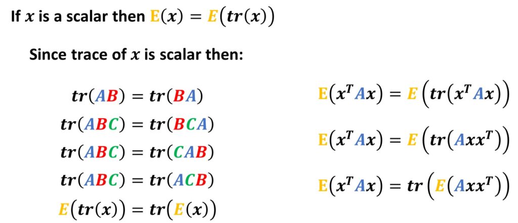
Now, we will consider the second term that has \(\mu_{2}\) and \(\Sigma_{2}\):

$$ \sum_{x}^{ }p\left ( x \right )\left [ \frac{1}{2}\left(x-\mu _{2}\right)^{\top} \Sigma_{2}^{-1}\left(x-\mu _{2}\right) \right ] $$

$$ \sum_{x}^{ }p\left ( x \right )\left \{ \frac{1}{2}\left[\left(x-\mu_{1}\right)+\left(\mu_{1}-\mu_{2}\right)\right]^{\top} \Sigma_{2}^{-1}\left[\left(x-\mu_{1}\right)+\left(\mu_{1}-\mu_{2}\right)\right] \right \} $$

The term that depends on \(\mu_{2}\) we extend, so that we get three terms by introducing \(– \mu_{1}\) and \(+ \mu_{1}\) in the expression:

$$ \sum_{x} p(x)\left [ \frac{1}{2}\left(x-\mu _{1}\right)^{\top} \Sigma_{2}^{-1}\left(x-\mu _{1}\right)+\frac{2}{2}\left(x-\mu _{1}\right)^{\top} \Sigma_{2}^{-1}\left(\mu_{1}-\mu _{2}\right)+\frac{1}{2}\left(\mu _{1}-\mu _{2}\right)^{T} \Sigma_{2}^{-1}\left(\mu _{1}-\mu _{2}\right) \right ] $$

$$ \Rightarrow E_{p}\left [\frac{1}{2}(x-\mu _{1})^{\top} \Sigma_{2}^{-1}(x-\mu _{1})+\left(x-\mu _{1}\right)^{\top} \Sigma_{2}^{-1}\left(\mu _{1}- \mu _{2}\right)+\frac{1}{2}\left(\mu _{1}-\mu _{2}\right)^{\top} \Sigma _{2}^{-1}\left(\mu _{1}-\mu _{2}\right) \right ] $$

And few more technical details …

$$E_{P}\left\{\frac{1}{2}\left(x-\mu_{1}\right)^{\top} \Sigma_{2}^{-1}\left(x-\mu_{1}\right)\right\}+E_{P}\left[\left(x-\mu_{1}\right)^{\top} \Sigma_{2}^{-1}\left(\mu_{1}-\mu_{2}\right)\right]+$$

$$+E_{P}\left[\left(\mu_{1}-\mu_{2}\right)^{T} \Sigma_{2}^{-1}\left(\mu_{1}-\mu_{2}\right)\right]=tr\left\{\frac{\Sigma_{2}^{-1} \Sigma_{1}}{2}\right\}+\left(\mu_{1}-\mu_{2}\right)^{\top} \Sigma_{2}^{-1}\left(\mu_{1}-\mu_{2}\right)+0 $$

$$ E_{p}\left[\left(x-\mu _{1}\right)^{\top} \Sigma_{2}^{-1}\left(\mu _{1}-\mu _{2}\right)\right] $$

$$ =\left [ \left ( E_{p}(x)-\mu_{1} \right )^{T}\Sigma _{2}^{-1}\left ( \mu _{1}-\mu _{2} \right ) \right ] = 0$$

Finally, we arrived to the final expression for the KL divergence:

$$ KL(P(x) \| Q(x))=\frac{1}{2}\left [ \log \frac{\left|\Sigma_{2}\right|}{\left|\Sigma _{1}\right|}-K+tr\left(\Sigma_{2}^{-1} \Sigma_{1}\right)+\left(\mu _{1}-\mu _{2}\right)^{\top} \Sigma_{2}^{-1}\left(\mu _{1}-\mu _{2}\right)\right ] $$

4. More insights into VAEs

Variational AutoEncoder: Working details of Variational AutoEncoder

In this part, we will continue our story about Variational Autoencoders. This will be a high-level overview and after this, we will explain all the mathematical details. 

We start with the block diagram of a variational autoencoder. Just to remind you, we have an input image \(x \) and we are passing it forward to a probabilistic encoder.

A probabilistic encoder is given with the function \(q_{\phi }\left ( z\mid x \right ) \). So, this is a conditional probability; \(x \) is the image and \(z \) is our latent vector. Here, we have a mean (\(\mu \)) and a standard deviation (\(\sigma \)). They are high dimensional probability parameters that VAE will learn. So, from this distribution, that we want to estimate, we will sample our latent vector \(z \). This vector, we will pass forward through a probabilistic decoder which is defined by the function of \(p_{\theta  }\left ( x\mid z \right ) \). We expect that the probabilistic decoder will give us the reconstructed image at the output. 

$$ Loss= L\left ( \theta ,\phi  \right )= -E_{z\sim q_{\phi }\left ( z\mid x \right )}\left [ p_{\theta }\left ( x\mid z \right ) \right ]+D_{KL}\left ( q_{\phi }\left ( z\mid x \right )\parallel p_{\theta }\left ( z \right ) \right ) $$

Next, let’s have a look at its cost function for the VAEs. Here, it is defined as the loss function of two parameters \(\theta \) and \(\phi \). Then, we have two terms. The first one is actually given with the mathematical expectation because in VAEs we work with probabilities. One reminder is that actually this mathematical expectation is an operator on the function \(q_{\phi }\left ( z\mid x \right ) \) and we want to find what is the mathematical expectation for term \(p_{\theta  }\left ( x\mid z \right ) \). So, this means that we are searching for the mathematical expectation of the expression inside the brackets given the probability distribution \(q_{\phi } \). And the second term is the Kullback-Leibler divergence. This term will tell us how much the two probability density functions are different. These two functions are again \(q_{\phi }\left ( z\mid x \right ) \) and \(p_{\theta }\left ( x\mid z \right ) \).

Now, we can ask ourselves what is actually the goal of variational autoencoders and why we actually use them?

Well, compared to traditional autoencoders we need to learn probabilistic distribution \(q_{\phi }\left ( z\mid x \right ) \). Once we learn the complete distribution, we would be able to sample from this distribution. Furthermore, we will be able to generate meaningful latent variables \(z \). 

The \(z \) vector in VAEs will not be fixed as we had for traditional autoencoders, but we can introduce subtle variation in this vector. Once we have a subtle variation, we have the possibility to reconstruct our image through a probabilistic decoder. Then, this image will not be actually in our training set but will be a very nice data representative. 

You can say “oh, this has indeed the similar properties as the images that we have in our set :-)”.

So, to state in the following way, the goal of VAEs is to find a distribution \(q_{\phi }\left ( z\mid x \right ) \) or some latent variable \(z \) from which we can sample \(z \) given distribution \(q_{\phi }\left ( z\mid x \right ) \) to generate new samples \({x}’ \).

So, what we showed with autoencoders is that actually, our latent variable \(z \) depends very much on the input data set. Somehow it is fixed. For instance, if we have MNIST data set, we will have 60, 000 images and that tells us that we would be able to reconstruct only 60, 000 latent vectors \(z \). However, imagine that for some of these vectors we introduced some subtle variations. We can increase vastly the number of data samples, preserving the “richness” and “variability” of the data samples.

So far, we don’t know how to do that, but let’s imagine that we do know. Then, we will have the overall probability distribution. Once we have a probability distribution, we are able to sample from this distribution, and then we would be able to generate a vector \(z \). For these latent vectors \(z \) once we pass them through a probabilistic decoder, we hope that we will get a sample, that is an image, that very much represents samples from this data set. For instance, we can get an image of the number 6. However, this digit is not present in a data set, but we are convinced that it is a number 6, and it would be difficult to tell for a human observer whether it is from our data set or not since it would be a realistic handwritten digit.

Now, let’s talk about latent variables in more detail.

Latent variables

One way to illustrate our vectors \(z \) is to study them with more focus and to see how they are connected with our image \(x \). First of all, we call them latent variables or hidden variables. In the previous block diagram, we saw that we cannot access these variables. They are also not labeled, but if we use this trick of the reconstruction loss we are able to indirectly estimate these values. This is the reason that we say that they are hidden. In this block scheme, we say that \(x \) is our observed variable and \(z \) is our latent variable. This also says that we want to discover a governing mechanism that is involved in the creation of the images. Then, this is linked with the probabilistic distribution \(p\left ( x\mid z \right ) \).

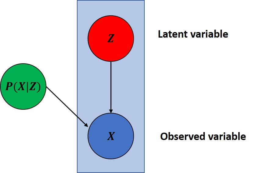
Moreover, it is important to note that the direction of the connection (link) is different and it depends on whether it goes from \(z \) to \(x \) or vice versa. Then, we have a probability \(p\left ( x\mid z \right ) \) and if it goes in the opposite direction we have a probability of \(p\left ( z\mid x \right ) \). So, these two are completely different probabilities.

Now, we will best understand the latent variables if we have a look at the following example. Latent variables correspond to real features of the object that are usually very difficult or tricky to be measured. For instance, let’s have a look at the image of a face. We can measure pixels. Easily, we can do this with a simple camera. Then, we will have access and we can read every RGB pixel value. However, in VAEs, this image is an input to the encoder. Then, we have our bottleneck or \(z \) latent vector. It is something that we cannot measure directly, but we can have a very concrete representation. So, for a face, we can have the following attributes that we would like to learn with VAEs. For instance, the elements of the vector \(z \) can be smile, skin tone, gender, beard, glasses, and hair color. For each of these, we will need to have a probabilistic distribution in order to fully create our variational autoencoder.

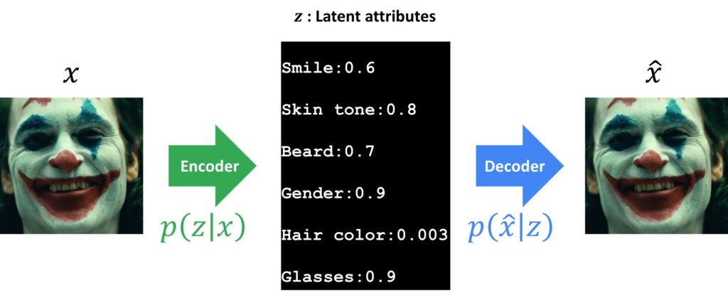
Finally, the goal of the probabilistic decoder will be to capture these latent vectors \(z \), and then, using the values that are stored in \(z \) give them certain expressions. So, as we can see here in our example, gender is \(0.9 \) and we can use this value to reconstruct our image in the output. Obviously, with such attributes, we want to have a reconstructed image of a male person. In addition, if the attribute for a smile is high, we will expect that in the reconstructed image a person is smiling.

Going deeper with this example, we can see one interesting thing about VAE. In case we want to train it, we have to bring to its input only images of faces. We better not mix categories. Now, it can be interesting to observe three different input images.

We can have a look at one single attribute and observe what is the difference between a traditional and variational autoencoder. Let’s say that we have three images and we can see for these three images that the smile is given by three fixed numbers. However, in a variational autoencoder, we will not have a fixed number, but we will get a probabilistic function as the output. And then, it will be close to the fixed number of autoencoders, but here from probabilistic distribution once we learn its parameters we will go and sample from it. Then, we will be able to get a reconstruction of our image that has a smile with this probability.

So, the VAE block diagram represents the encoder and decoder part and in between, we have a learned probabilistic multivariate distribution. For each of these attributes, we actually learn \(\mu \) and \(\sigma \) values and we assume that they are Gaussian distributions. So, what will actually happen is that we will sample from these distributions and we will be able to generate new generative models that the decoder will have to reconstruct for us. In this way, we will not use fixed values as with the traditional autoencoder, but with these new values, we can generate new data that have a lot of potential. 

5. Derivation of the Loss Function

In order to define and optimize loss function for variational autoencoders, we will use the concept called the problem of approximate inference. So, what is this? Well, let’s suppose that we have a vector \(x \), and let vector \(x \) be an observable variable. In this case, with the variational autoencoders, \(x \) is an input image. We also define \(z \) as a set of latent variables. For these two variables \(x \) and \(z \) we define a joint distribution. This joint distribution is defined as a probability density function written as \(p\left ( z,x \right ) \). Defined in this way, the conditional distribution of latent variables \(p\left ( z\mid x \right ) \) is then given with the following formula:

$$ p(z | x)=\frac{p(x | z) p(z)}{p(x)} $$

If we use a Bayes’ formula, we can express \(p\left ( z\mid x \right ) \). However, there is one problem with this formula. It is difficult to be solved. The reason for this is because \(p\left (x \right ) \) is not known. Why is \(p\left (x \right ) \) unknown? A reason is that we have an integral that we integrate over \(z \) and we have a formula that says:

$$ p(x)=\int p(x | z) p(z) d z=\int p(x, z) d z $$

This integral cannot be so solved. We say that such an integral is intractable. That means that actually, it requires the exponential time to be computed. This is due to the fact that the multiple integrals are involved for latent variable \(z \) vector.

We say that this is intractable to be solved as we will need to integrate over the number of elements that we have in a latent variable \(z \). So, for instance, in our previous examples with the faces, we had six attributes for our latent vector. This would mean that we will have to integrate the joint distribution six times. We will have six integrals. And that’s not easy to solve! Moreover, they also do not have an explicit formula for \(p\left ( z,x \right ) \), and therefore, this is actually impossible to be solved in a closed-form.

Now, we need to find the solution for this. An alternative is actually not to use \(p\left ( z\mid x \right ) \), but to use another distribution \(q\left ( z\mid x \right ) \). And in this way, we want this distribution to be defined so that it has a tractable solution. This can be achieved using variational inference.

The main idea is that we will actually model distribution \(p\left ( z\mid x \right ) \) with \(q\left ( z\mid x \right ) \). Since \(p\left ( z \right ) \) can be very difficult to express numerically we will try to approximate it with something that’s very easy to calculate. A probability distribution that’s very common and relatively easy to be used for calculation is the Gaussian distribution. So, we will model \(q\left ( z\mid x \right ) \) as a probabilistic Gaussian distribution. We will use the following term that’s KL divergence and this measure will assist us to model the difference between two probability distributions \(p\left ( z\mid x \right ) \) and \(q\left ( z\mid x \right ) \). The following formula explains how actually KL is calculated and we have already derived this in much detail in our previous paragraphs.

$$ D_{K L}\left(q_{\phi }(z \mid  x) \parallel p_{\theta }(z \mid x)\right)=\sum_{z} q_{\phi }(z \mid  x) \log \left(\frac{q_{\phi }(z \mid x)}{p_{\theta}(z \mid x)}\right) $$

 $$ = E_{z\sim q_{\phi }\left ( z\mid x \right )}\left[\log \left(\frac{q_{\phi }(z \mid x)}{p_{\theta }(z \mid x)}\right)\right] $$

 $$ = E_{z\sim q_{\phi }\left ( z\mid x \right )}[\log (q_{\phi }(z \mid  x))-\log (p_{\theta }(z \mid x))] $$

$$ D_{K L}\left[q_{\phi }(z \mid  x) \parallel p_{\theta }(z \mid x)\right]=E_{z}\left[\log q_{\phi }(z \mid  x)-\log \frac{p_{\theta }(x \mid z) p_{\theta }(z)}{p_{\theta }(x)}\right] $$

$$ = E_{z}\left[ log(q_{\phi}(z | x))-log(p_{\theta}(x | z))-log p_{\theta}(z)+log p_{\theta}(x)\right] $$

$$ D_{K L}\left[q_{\phi }(z \mid  x) \parallel p_{\theta }(z \mid x)\right]-\log p_{\theta }(x)=E_{z}\left [ \log q_{\phi }(z\mid x)-\log p_{\theta}(x\mid z)-\log p_{\theta }(z) \right ] $$

By using KL divergence as a measure for the difference between two distributions we can now cast our optimization problem. So, if we can set up an optimization problem to minimize KL divergence between probabilities \(p \) and \(q \) and if we manage to calculate our parameters \(\theta \) and \(\phi \) we would be able to get a very good approximation of \(p \)  with the \(q \) probability distribution. In the following formula, it can be seen that the equations actually expressed this. Using the previous equations, we can also substitute the first formula in the second formula, and then, we will get a new formula that is expressed by substituting part of \(p \) as a conditional distribution. Hence, we will get a slightly improved formula for the KL divergence.

Finally, we can express KL as an expectation operator over the last variable \(z \). Here, \(z \) is sampled from \(q_{\phi }\left ( z\mid x \right ) \) and we have to calculate the mathematical expectation of a formula given in brackets. The last term that we see here is \(\log p_{\theta }\left ( x \right ) \). This term does not depend on \(z \), therefore, it can be treated as a simple constant and we can remove it from the expression. So, we can simplify our equation a little bit, and we can subtract this term from KL and we will get an expectation of \(z \) over a modified expression.

$$ \log p_{\theta }(x)-D_{K L}\left[q_{\phi }(z \mid  x)\parallel p_{\theta }(z \mid x)\right] $$

$$ = E_{z}[\log (p_{\theta }(x \mid z))]-E_{z}\left[\log q_{\phi }(z\mid x) -\log   p_{\theta }(z)\right] $$

$$ = E_{z}[\log (p_{\theta }(x \mid z))]-D_{K L}\left[q_{\phi }(z\mid x) \parallel  p_{\theta }(z)\right] $$

We can now proceed and rearrange the previous equations by putting a minus sign in front of them. Then, we will actually obtain the formula that consists of two terms. One will be the expectation of a logarithm of the probability function \(p_{\theta }\left ( x\mid z \right ) \) over variable \(z \). Then we have a minus KL of the two probabilities: 1) \(q_{\phi } \) and 2) \(p_{\theta } \). So, basically, we see that the optimization function that we need to minimize consists of two terms. The first one is the reconstruction likelihood. So, this means that we want to have a very small reconstruction error. On the other hand, we want to learn the function \(q_{\phi } \) to be as close to the function \(p_{\theta }\left ( z \right ) \). This \(p \) is a priori distribution function.

$$ L(\theta, \phi)=-E_{z \sim Q_{\phi }(z / x)}[\log (p_{\theta } (x \mid  z))]+D_{K L}\left[Q_{\phi}(z \mid x) \parallel p_{\theta }(z)\right] $$

$$ \log p_{\theta}(x)-D_{K L}\left[Q_{\phi}(z \mid  x) \parallel p_{\theta }(z | x)\right]=-L(\theta , \phi) $$

Note that a loss function represents an objective function that we want to minimize with the minus sign in front of it. And we get the loss function with parameters \(\theta \) and \(\phi \). So, this is the function that we will need to optimize.

Interesting thing is that these two terms are reconstruction terms in the regulariser. We don’t need to introduce a new regularization term into our loss function, as it is already provided via the KL part. So, let us recall that \(L \) depends on a \(\theta \) and \(\phi \) and what we want to do is to minimize the loss function. In return, this will optimize parameters \(\theta ^{\ast } \) and \(\phi ^{\ast } \). These parameters are actually the weights of two neural networks that we want to learn.

Now, we will provide a little bit more intuition about the loss function. As you can see it is given by two terms depending on parameters \(\theta \) and \(\phi \). What we can see is that the first term is a mathematical expectation with parameter \(z \) over a log of probabilistic function. This term can also be seen as a log-likelihood term. Why is that? Because \(p_{\theta }\left ( x\mid z \right ) \)  can be seen as Gaussian or normal distribution with parameters \(\mu _{\theta }\left ( z \right ) \) and \(\Sigma _{\theta }\left ( z \right ) \). When we take the logarithm of the Gaussian function we get the square error between the data sample \(x \) and a mean of the Gaussian distribution. Hence, we will have \(q_{\phi }\left ( z\mid x \right ) \) and this is called a recognition model and it maps \(x \) into \(z \).

$$ p_{\theta }\left ( x\mid z \right ) = N\left ( \mu _{\theta }\left ( z \right ),\Sigma_{\theta }\left ( z \right )  \right ) $$

The following formula can be expressed as a multivariable Gaussian function and it is defined with the covariance matrix \(\mu _{\theta }\left ( z \right ) \). Once we take a logarithm of this probabilistic function \(p_{\theta }\left ( x\mid z \right ) \) we will obtain actually a term \(x-\mu _{\theta }\left ( z \right ) \). So, this term along with the remaining part can be seen as the squared reconstruction error. In addition, this term is also called the data fidelity in inverse problem.

$$ p_{\theta}(x | z)=\frac{1}{\sqrt{(2 \pi)^{k}\left|\Sigma_{\theta}(z)\right|}} \exp \left[\frac{\left(x-\mu _{\theta}(z)\right)^{T} \Sigma _{\theta}^{-1}{(z)}\left(x-\mu_{\theta}(z)\right)}{2}\right] $$

$$ \log p_{\theta }(x \mid  z) \sim \left(x-\mu _{\theta }(z)\right)^{T} \Sigma_{\theta }^{-1}(z)\left(x-\mu _{\theta }(z)\right) $$

On the other hand, we also have this second term \(D_{KL} \). We should call this term a regulariser. Basically, that’s a KL divergence between the \(q_{\phi }\left ( z\mid x \right ) \) and the function \(p_{\theta }\left ( z \right ) \). So, here \(p_{\theta }\left ( z \right ) \) is a Gaussian prior function, and basically, \(D_{KL} \) should tell us how far away these probabilistic functions are from each other.

Now we will just discuss a little bit more in detail the choice of our probability density function. Here, we have the Gaussian probability of a mean value zero and a standard deviation of one. This is the reason because we want our p_{\theta }\left ( z \right ) $ to be very close to \(q_{\phi }\left ( z\mid x \right ) \). This means that actually we really want to insist that there is a variance present in this distribution and we don’t want to have a narrow distribution.

On the other hand, if we choose \(p_{\phi }(z)= \mathcal{N}(0,1) \), we have one more benefit. We can say that we want \(q_{\phi }\left ( z\mid x \right ) \) to be Gaussian with parameters \(\mu _{\phi }(x) \) and \(\Sigma_{\phi }(x) \). This means that we will have a closed form for KL divergence, and this was already derived in the previous paragraph.

$$ KL(p (x)\parallel q(x))=\frac{1}{2}\left [ \frac{\left | \Sigma _{2} \right |}{\left | \Sigma _{1} \right |}-K+tr(\Sigma _{2}^{-1},\Sigma _{1})+(\mu _{1}-\mu _{2})^{T}\Sigma _{2}^{-1}(\mu _{1}-\mu _{2}) \right ] $$

Hence, if we recall we will have the function that’s derived for two arbitrary Gaussian distributions. Now, we will have the coefficients: \(\Sigma _{1} \) will be \(\Sigma_{\phi }\left ( x \right ) \), \(\Sigma_{2}\) will be one and \(\mu _{2} \) will be equal to zero. Now, once we plug in these values \(\mu \) will be \(\mu _{\phi }\left ( x \right ) \) as you can see in the following formula. At last, we now achieve the final result. It’s relatively simple and it depends on \(\mu _{\phi } \) and \(\Sigma_{\phi } \). One important parameter here is \(K \) and that’s the dimensionality of our \(z \) vector.

$$ D_{K L}\left [ \mathcal{N}(\mu _{\phi }(x),\Sigma _{\phi }(x))\parallel \mathcal{N}(0,1) \right ]= $$

$$ \frac{1}{2}\left[tr\left(\Sigma _{\phi }(x)\right)+\mu_{\phi }(x)^{T} \mu _{\phi }(x)-K-\log |\Sigma _{\phi }(x)|\right] $$

In addition, we will also have a term \(\left | \Sigma _{\phi }\left ( x \right ) \right | \). This is a simple trace function which is the sum of diagonal elements of a matrix \(\Sigma _{\phi }(x) \). In addition, we have a determinant of \(\Sigma _{\phi }(x) \) and because \(\Sigma \) is a diagonal matrix it can be written in a very simplified term.

$$ D_{K L}\left [ \mathcal{N}(\mu _{\phi }(x),\Sigma _{\phi }(x))\parallel \mathcal{N}(0,1) \right ]= $$

$$= \frac{1}{2}\left(\sum_{K} \Sigma _{\phi }(x)+\sum_{K} \mu _{\phi }^{2}(x)-\sum_{K} 1-\log  \prod_{K}^{ }\Sigma {\phi }(x)\right) $$

$$ =\frac{1}{2}\left(\sum_{K} \Sigma _{\phi }(x)+\sum_{K} \mu _{\phi }^{2}(x)-\sum_{K} 1-\sum_{K} \log \left(\Sigma {\phi }(x)\right)\right) $$

$$ =\frac{1}{2} \sum_{K}\left(\Sigma _{\phi }(x)+\mu _{\phi }^{2}(x)-1-\log \left(\Sigma _{\phi  }(x)\right)\right) $$

$$ D_{K L}\left[N\left(\mu _{\phi}(x), \Sigma _{\phi}(x)\right)\parallel N(0,1)\right]=\frac{1}{2} \sum_{K}\left [ \exp (\Sigma {\phi }(x)\right)+\mu _{\phi}^{2}(x)-1-\Sigma _{\phi }(x)] $$

So, finally we obtain the final loss for a Variational Autoencoder!!!

$$ L(\theta, \phi )=-E_{z}\left[\log \left(\mu _{\theta }(x \mid  z)\right)\right]+\frac{1}{2} \sum_{K}\left[\exp \left(\Sigma _{\phi }(x)\right)+\mu _{\phi }^{2}(x)-1-\Sigma_{\phi }(x)\right] $$

6. Optimization and Reparameterization Trick

$$ \log p(\theta )-D_{K L}\left[Q_{\phi}(z \mid  x) \parallel p_{\theta }(z \mid x)\right]=-L(\theta, \phi) $$

In the final part of this post, we will discuss how to optimize the cost function for variational autoencoders. That means that we want to minimize our loss function that depends on the parameters \(\theta \) and \(\phi \). One thing that we will explore here, is that actually in the variation method, the loss function is known as the variational lower bound on evidence or evidence lower bound, the so-called ELBO. This lower bound part is due to the fact that KL divergence is always non-negative, and therefore, it will represent a lower bound for the loss function \(L(\theta,\phi ) \).

$$ D_{K L}[q_{\phi }(z \mid  x) \parallel p_{\theta }(z \mid x)] \geq 0 $$

$$ L(\theta, \phi) \leq \log p_{\theta }(x) $$

Therefore, by minimizing the loss, we are maximizing the lower bound of the probability function to generate real data samples.

$$ L(\theta, \phi)=-E_{z \sim q_{\phi }(z \mid  x)}[\log (p_{\theta } (x \mid  z))]+\frac{1}{2}\sum_{K}\left [ exp\left ( \Sigma _{\phi } (x)\right )+\mu _{\phi }^{2}(x)-1-\Sigma _{\phi }(x) \right ] $$

$$ \theta^{*}, \phi^{*}= argmin L(\theta , \phi) $$

 So, in order to achieve this optimization we have a strategy for the optimization. What we will use to optimize it is the so-called alternate optimization principle.

1. $$ \theta^{*}=\nabla_{\theta }\{L(\theta , \phi)\} $$
   • $$ \phi = constant $$
2. $$ \phi ^{*}=\nabla_{\phi  }\{L(\theta , \phi)\} $$
   • $$ \theta= constant $$

We have two sets of parameters. First, we will try to find an optimal vector \(\theta ^{\ast } \). In order to do that we will find the partial derivative of our loss function. In this way, we will treat the \(\phi \) as a constant. This will give us value for \(\theta ^{\ast } \), and afterwards in the subsequent step, we will actually calculate \(\phi ^{\ast } \) as a partial derivative with respect to \(\phi \) of the loss function. So, the values that we will use then in the loss function would be \(\theta ^{\ast } \) values calculated in the previous step.

Next, we will repeat this step several times. This number of alterations will be defined with the iterator that can go from 1 to 10. In each of these steps we first calculate \(\theta \), then we go to the following step and we calculate \(\phi \) using this calculated \(\theta ^{\ast } \). Then, we go back again and calculate \(\theta \) which is like an update of \(\theta \). We will repeat this until we finally calculate two final parameters (or a set of parameters) that we will use in the final model.

One important thing to note here is that once we are calculating a partial derivative with respect to \(\theta \), usually we do not have any problems encountered. However, once we perform a derivation with respect to \(\phi \) we will encounter some problems and we will see how actually we can cope with this.

$$ L(\theta, \phi)=-E_{z \sim Q_{\phi }(z / x)}[\log (p_{\theta } (x \mid  z))]+\frac{1}{2}\sum_{k}\left [ exp\left ( \Sigma _{\phi } (x)\right )+\mu _{\phi }^{2}(x)-1-\Sigma _{\phi }(x) \right ] $$

$$ \hat{\theta}_{i}=\nabla_{\theta} L(\theta, \phi) $$

$$ \hat{\theta}_{i}=\nabla_{\theta} \left \{ -E_{z \sim q_{\phi }(z | x)}[\log (p_{\theta } (x \mid  z))]+\frac{1}{2}\sum_{k}\left [ exp\left ( \Sigma _{\phi } (x)\right )+\mu _{\phi }^{2}(x)-1-\Sigma _{\phi }(x) \right ]  \right \} $$

We will perform the following reparameterization trick in order to solve this. We will do the optimization with respect to both \(\theta \) and \(\phi \) and we would like to learn functions \(q_{\phi }\left ( z\mid x \right ) \) and \(p_{\theta }\left ( x\mid z \right ) \) simultaneously. So, this will be the loss function that we have from before. It is written here, and we actually want to minimize it by using parameters \(\theta \) and \(\phi \). So, we will alternate these two derivatives with respect to \(\theta \) and \(\phi \), and then as we discussed already we will come to the corresponding solution. So, once we perform derivatives with \(\theta \) as we can see, we will get the following expression here. 

$$ \hat{\theta}_{i}=\nabla_{\theta} L(\theta, \phi) $$

$$ \hat{\theta}_{i}\cong \frac{1}{L} \sum_{l=1}^{L} \nabla_{\theta} \log p_{\theta}\left(x \mid  z^{(l)}\right) $$

$$ z^{(l)} \sim Q_{p}(z \mid  x) $$

One interesting thing to note here is that the expected term is now replaced with the Monte Carlo estimate. This means that we have replaced expectation with the sum where the number of samples goes from 1 to \(L \). These are values for our vector \(z^{(l)} \). That means that \(z^{(l)} \) is sampled from the distribution \(q_{\phi }\left ( z\mid x \right ) \).

$$ \hat{\phi }_{i}=\nabla_{\phi } L(\theta, \phi) $$

$$ \nabla_{\phi} E_{Q_{\phi}(z\mid x)}[f(z)] \neq E_{Q_{\phi}(z\mid x)}\left[\nabla_{\phi} f(z)\right] $$

That was the calculation for \(\hat{\theta }_{i} \). Now, we will continue to derive for \(\hat{\phi}_{i} \) the derivative of the loss function by taking \(\theta \) as a constant.

As you can see we will encounter a problem that’s shown here in the following equation because we need to take a partial derivative of the expectation function with the respect to \(\phi \).

The problem is that this expectation function is inside the term. So, basically \(z \) is distributed from \(q_{\phi }\left ( z\mid x \right ) \). Therefore, the derivative of \(\phi \) is very hard to estimate because \(\phi \) appears in the distribution with respect to which the expectation is taken. In simple words, the partial derivative of \(\phi \) cannot just enter into the expectation because the expectation itself depends on the function \(q_{\phi }\left ( z\mid x \right ) \).

Hence, our solution to this would be to actually move expectations with respect to this function inside the term in the brackets. This is possible to be done. So, basically we will create one linear transformation so that \(z=g_{\phi }\left ( \epsilon , x \right ) \) where \(\epsilon \) is a normal distribution with a zero mean and a standard deviation of one. In this way, we can remove our dependence from the expectation operator that we will show in the following step.

$$ E_{Q_{\phi}(z \mid  x)}[f(z)]=E_{p(\epsilon )}\left[f\left(g_{\phi}(\epsilon, x)\right)\right] $$

$$ g_{\phi }(\epsilon, x)=\mu_{\phi}(x)+\epsilon \odot \Sigma _{\phi }^{1 / 2}(x)=z\sim N\left ( \mu (x),\Sigma (x) \right ) $$

As we see in this transformation we are transforming a function \(g_{\phi }\left ( \epsilon , x \right ) \) and we transform it into \(\mu _{\phi }(x) \) plus \(\Sigma (x) \) times square root of the covariance matrix with respect to dependent \(x \). This transformation is a very classical procedure that’s used in probability. In this way our sampling vector is again a Gaussian variable. Its mean value is \(\mu (x) \) and \(\Sigma (x) \) is a covariance matrix. In other words, we actually create one Gaussian distribution using the normalised Gaussian distribution.

$$ z= \mu_{\phi}(x)+\epsilon \odot \Sigma _{\phi }^{1 / 2}(x) $$

Now, instead of sampling \(z \) from the function \(q_{\phi }\left ( z\mid x \right ) \) we can sample from the normal distribution \(N(0, 1) \) and using the linear transformation we eventually get the same vector \(z \) as a combination of \(\mu _{\phi }(x) \) and \(\epsilon \) that multiplies \(\Sigma _{\phi }(x) \). This is represented now in our updated block diagram where actually we see that \(z \) now equals \(\mu \) plus $latex\epsilon $ times \(\Sigma \). This is a so-called reparameterization trick that has been applied. We can see this in the image below. First of all, we have that the \(z \) is a stochastic sampling vector from the function \(q \). Indeed, it depends on \(\phi \) and \(x \). The following image illustrates the original and reparametrized form.

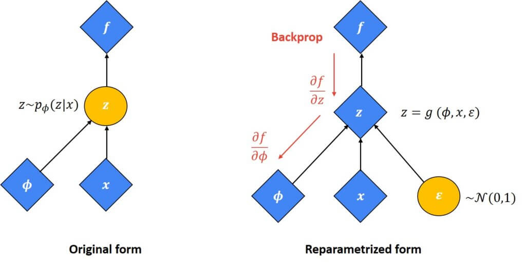
In this reparameterized form, \(z \) now depends on these three parameters. We can take derivatives with respect to these parameters. This is something that we won’t calculate, and therefore, it is important that we are able to take a derivative with respect to \(\phi \). On the other hand, we still have that \(z \) depends on \(\epsilon \), but somehow it is now removed from this part. Finally, we can actually obtain our gradient and perform a backpropagation step.

If we now write the expression for the \(\hat{\phi}_{i} \) which is like a derivative of a loss function with respect to \(\phi \) by keeping \(\theta \) constant we saw that actually we cannot plug in this derivative operator inside the expectation.

However, with this modified approach we have actually managed to create our latent vector \(z^{(l)}\sim p\left ( \epsilon  \right ) \) and we have actually removed the \(\phi \) parameters from the expression. Hence, this will be a modified expression for \(\hat{\phi}_{i} \) and if we continue solving this we can see that actually we can obtain the desired equation. Now, finally, we have an expression where derivative with respect to \(\phi \) is plugged in into the expectation term. This is the resulting equation that we can see.  

$$ \hat{\phi }_{i}=\nabla_{\phi } L(\theta, \phi) $$

$$ =\nabla_{\phi }=\left \{ -E_{z \sim q_{\phi }(z / x)}[\log (p_{\theta } (x \mid  z))]+\frac{1}{2}\sum_{k}\left [ exp\left ( \Sigma _{\phi } (x)\right )+\mu _{\phi }^{2}(x)-1-\Sigma _{\phi }(x) \right ] \right \} $$

$$ =\nabla_{\phi }=\left \{ -E_{z^{(l)} \sim p(\epsilon )}[\log p_{\theta } (x \mid  z^{(l)})]+\frac{1}{2}\sum_{k}\left [ exp\left ( \Sigma _{\phi } (x)\right )+\mu _{\phi }^{2}(x)-1-\Sigma _{\phi }(x) \right ] \right \} $$

$$ \hat{\phi }_{i}=-E_{z^{(l)} \sim p(\epsilon )}[ \nabla_{\phi }\left ( \log p_{\theta }(x \mid  z^{(l)}) \right )]+\nabla_{\phi }\left [ \frac{1}{2}\left ( \sum_{k}\left [ exp(\Sigma _{\phi }(x))++\mu _{\phi }^{2}(x)-1-\Sigma _{\phi }(x) \right ]\right )\right ] $$

$$ =\frac{-1}{L} \sum_{l=1}^{L} \cdot\left[\log p_{\theta}\left(x \mid  z^{(l)}\right)\right] $$

Finally, with the alternating optimization technique, we can have an estimate of this parameter and we can then proceed with the calculation of the optimal parameters \(\theta \) and \(\phi \). So, that means that we managed to get rid of this problem that we faced earlier. All this is given in the equations in the slides and this finally concludes the theoretical part of variational autoencoders.  

Summary

We do not give a summary for this post 🙂 This was a long one. Actually, the longest we have ever written. Our goal was to show that there is no magic here involved and that we can track all the details just if we show a little bit of effort and persistence. In the next post, we will show practical steps how to implement VAE in PyTorch. Now, we are ready to start with the Generative Adversarial Networks.