OpenCV #005 Averaging and Gaussian filter

Digital Image Processing using OpenCV (Python & C++)
Highlights: In this post, we will learn how to apply and use an Averaging and a Gaussian filter. We will also explain the main differences between these filters and how they affect the output image.
What does make a good filter? This is a million dollar question.
Tutorial Overview:
1. Averaging filter
What does make a good filter? So, let’s start with a box filter. In the Figure below, we see the input image (designed from numbers) that is processed with an averaging filter. We also say box/uniform/blur, and yes, these are all synonyms :-). Here, all the coefficient values have the same weight. That is, the averaging filter is a box filter of all coefficients having the value \(\frac{1}{9} \).

\(F (x, y) \) and the result
\(G (x, y) \) is what we got
Now, as the filter \(H (u, v) \) is being moved around the image \(F (x, y) \), the new image \(G (x, y) \) on the right is generated.
Next, let’s say that we process an image below with the averaging box filter. What should we expect as a result? Well, we will get an ugly image like the one on the right.

An image on the left is visually applealing and the image is quite smooth. However, the generated image looks nothing like it. There are some unnatural sharp edges at the output \(G (x, y) \).
What was problematic with that? The square is not smooth! Trying to blur or filter an image with a box that is not smooth does not seem right. When we want to smooth an image our goal is to catch the significant pieces of the information (lower frequency content). Subsequently, we will see that a better result will be obtained with a Gaussian filter due to its smoothing transitioning properties.
Code for Averaging filter
Python
Both in Python and C++ averaging filter can be applied by using blur() or boxFilter() functions.
C++
#include <iostream>
#include <opencv2/opencv.hpp>


using namespace std;
using namespace cv;

int main() {

    cv::Mat image = imread("car.jpg", IMREAD_GRAYSCALE);
    cv::Mat processed_image;

    // we create a simple blur filter or an average/mean filter
    // all coefficients of this filter are the same
    // and this filter is also normalized.


    cv::imshow("Original image", image);
    cv::blur(image, processed_image, Size(3,3) );
    cv::waitKey();

    cv::imshow("Blur filter applied of size 3", processed_image);
    cv::waitKey();

    cv::blur(image, processed_image, Size(7,7));
    cv::waitKey();

    cv::imshow("Blur filter applied of size 7", processed_image);
    cv::waitKey();


    // Here we create an image of all zeros.
    // Only one pixel will be 1.
    // In this example we will generate a very small image so that we can
    // better visualize the filtering effect with such an image.

    cv::Mat image_impulse = cv::Mat::zeros(31, 31, CV_8UC1);
    image_impulse.at<uchar>(16,16) = 255;


    image_impulse = image_impulse * 20;
    cv::imshow("Impulse image", image_impulse);
    cv::waitKey();

    cv::Mat image_impulse_processed;


    cv::blur(image_impulse, image_impulse_processed, Size(3,3));
    image_impulse_processed = image_impulse_processed * 20;
    cv::imshow("Impulse image", image_impulse_processed);
    cv::waitKey();

    // this will produce a small square of size 3x3 in the center
    // Notice that, since the filter is normalized,
    // if we increase the size of the filter,
    // the intensity values of the square in the output image will be more lower. \
    // Hence, more challenging to be detected.


    cv::blur(image_impulse, image_impulse_processed, Size(7,7));
    image_impulse_processed = image_impulse_processed * 20;
    cv::imshow("Impulse image", image_impulse_processed);
    cv::waitKey();
Let’s see the results of our code:

Interestingly, when we do filtering, the larger the kernel size, the smoother the new image would be. Here below is a sample of filtering an impulse image (to the left), using a kernel size of 3×3 (in the middle) and 7×7 kernel size (to the right).

2. Gaussian filter
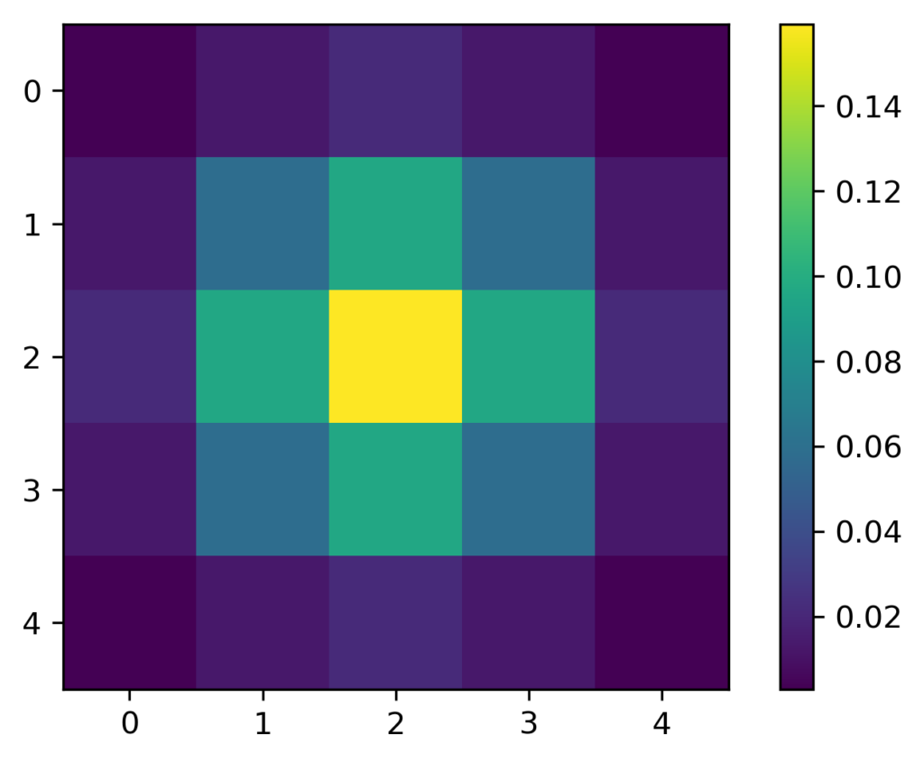
So, we all know what a Gaussian function is. But how will we generate a Gaussian filter from it? Well, the idea is that we will simply sample a 2D Gaussian function. We can see below how the proposed filter of a size 3×3 looks like.

Using the \(3\times 3 \) filters is not necessarily an optimal choice. Although we can notice its higher values in the middle that falls off at the edges and even more at the corners, this can be considered as a poor representation of the Gaussian function.
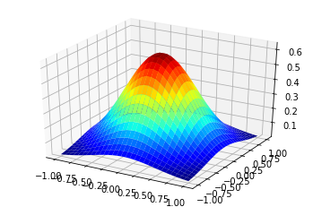
Here, we plot a Gaussian function both in 2D & 3D so we gain more intuition how larger Gaussian filters will look like:
\(h \left ( u,v \right )= \frac{1}{2\pi \sigma ^{2}} e^{-\frac{u^{2}+v^{2}}{\sigma ^{^{2}}}} \)


Here, we can refresh our knowledge and write the exact formula of Gaussian function:
\(\exp (-\frac{ (x^{2}+y^{2}) }{2\sigma ^{2}}) \)
Next, if we take an image and a filter it with a Gaussian blurring function of size 7×7 we would get the following output.

Wow! So, much nicer. Compare smoothing with a Gaussian to the non-Gaussian filter to see the difference.

In the non-Gaussian, we see all those sharp edges. When compared with the Gaussian, we get a nice smooth, blur on the new image.
Code for Gaussian filter
Python
C++
// Gaussian filter

    // First we will just apply a Gaussian filter on the image
    // this will also create a blurring or smoothing effect..
    // Try visually to notice the difference as compared with the mean/box/blur filter.


    cv::Mat image_gaussian_processed;
    cv::GaussianBlur(image, image_gaussian_processed, Size(3,3), 1);
    cv::imshow("Gaussian processed", image_gaussian_processed);
    cv::waitKey();

    cv::GaussianBlur(image, image_gaussian_processed, Size(7,7), 1);
    cv::imshow("Gaussian processed", image_gaussian_processed);
    cv::waitKey();
Output

Smoothing with a 7×7 Gaussian filter on the right
Python
C++
cv::Mat image_impulse_gaussian_processed;
    cv::GaussianBlur(image_impulse, image_impulse_gaussian_processed, Size(3,3), 1);
    image_impulse_gaussian_processed = image_impulse_gaussian_processed * 20;
    cv::imshow("Gaussian processed - impulse image", image_impulse_gaussian_processed);
    cv::waitKey();

    cv::GaussianBlur(image_impulse, image_impulse_gaussian_processed, Size(9,9), 1);
    // here we have just multiplied an image to obtain a better visualization
    // as the pixel values will be too dark.
    image_impulse_gaussian_processed = image_impulse_gaussian_processed * 20;
    cv::imshow("Gaussian processed - impulse image", image_impulse_gaussian_processed);
    cv::waitKey();
Output

Python
C++
// here we will just add random Gaussian noise to our original image

    cv::Mat noise_Gaussian = cv::Mat::zeros(image.rows, image.cols, CV_8UC1);

    // here a value of 64 is specified for a noise mean
    // and 32 is specified for the standard deviation

    cv::randn(noise_Gaussian, 64, 32);

    cv::Mat noisy_image, noisy_image1;

    noisy_image = image + noise_Gaussian;
    cv::imshow("Gaussian noise added - severe", noisy_image);
    cv::waitKey();

    //adding a very mild noise
    cv::randn(noise_Gaussian, 64, 8);
    noisy_image1 = image + noise_Gaussian;
    cv::imshow("Gaussian noise added - mild", noisy_image1);
    cv::waitKey();
Output

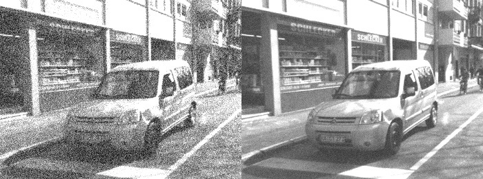
And a medium Gaussian noise was added to the right image
Python
C++
// Let's now apply a Gaussian filter to this.
    // This may be confusing for beginners.
    // We have one Gaussian distribution to create a noise
    // and other Gaussian function to create a filter, sometimes also called a kernel.
    // They should be treated completely independently.

    cv::Mat filtered_image;
    cv::GaussianBlur(noisy_image, filtered_image, Size(3,3), 3);
    cv::imshow("Gaussian noise severe - filtered", filtered_image);
    cv::waitKey();

    cv::GaussianBlur(noisy_image1, filtered_image, Size(7,7), 3);
    cv::imshow("Gaussian noise mild - filtered", filtered_image);
    cv::waitKey();


    return 0;
}
Output

Summary
Finally, we have learned how to smooth (blur) an image with a Gaussian and non-Gaussian filter. We realize why it is preferable to use a Gaussian filter over a non-Gaussian one. In the next posts, we will talk more about Sobel operator, image gradient and how edges can be detected in images.