#023 PyTorch - DeepLab v3+ for Semantic Segmentation in PyTorch

#023 PyTorch – DeepLab v3+ for Semantic Segmentation in PyTorch

datahacker.rs PyTorch 03.01.2022 | 0

Highlights: The year 2017 was very fruitful for Google researchers working on semantic segmentation. Their proposed model called the DeepLab was significantly improved over several iterations. In their 4th paper, they present Version 3+ of the same model.

In this blog post, we will study the theoretical novelties of this version that utilizes the model developed and popularized in Version 2. We will also see how they frame the first model as the decoder part and add a novel encoder part where they employ the Xception model and depth-wise separable convolution. We will also dive into coding a full network in PyTorch. So let us begin!

Tutorial Overview:

Introduction to DeepLab v3+
The Encoder part
The Decoder part
DeepLab v3+ Implementation in PyTorch

1. Introduction to DeepLab v3+

In 2017, two effective strategies were dominant for semantic segmentation tasks. One was the already introduced DeepLab that used atrous (dilated) convolution with multiple rates. The second strategy was the use of encoder-decoder structures as mentioned in several research papers that tackled semantic segmentation. U-Net is one such example.

DeepLab v3+ proposed to combine the best sides of both approaches by:

Keeping their original atrous convolution part with multiple rates, and practically transforming it into a decoder part, also known as Atrous Spatial Pyramid Pooling block (ASSP).
Introducing a simple but effective decoder designed on the Xception architecture combined with the depth-wise separable convolution.

All this resulted in a faster and stronger network. The first part encapsulated rich contextual information, whereas the second one recovered spatial information and accurately segmented object boundaries. This model, at the time of the publishing, achieved state-of-the-art results on several datasets.

Have a look at the pictorial overview of the model in the image below:

In the image above, we can see the following steps:

Spatial pyramid pooling: This is the decoder part with atrous convolution with multiple rates.
Encoder-Decoder: The encoder part gradually reduces the feature maps while capturing the semantic information of the image content. On the other hand, the goal of the decoder is to gradually recover the spatial information to allow the precise segmentation of boundaries.
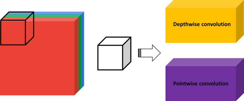
Depth-wise Separable Convolution: This is quite interesting and we shall go into more details to understand and demonstrate that the amount of multiplications in convolutional layer, can actually be relatively large.

The first point to note is that depth-wise separable convolution consists of an additional block: point-wise convolution.

Assume that we have the following convolution operation. The input feature map is of size \(12\times12\times3 \), whereas the kernel/filter is of size \(5\times5\times3 \) . The total amount of needed multiplication operations are shown in the following image:

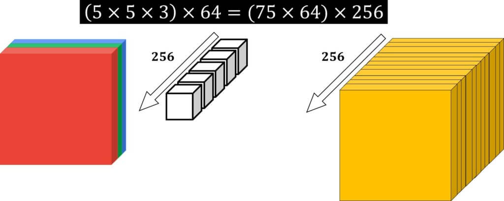
For a single output element processing, we have \(5\times5\times3 \) multiplications. Then, if there is no zero padding, the output feature map will be of size \(8\times8 = 64 \) elements. And, if we assume that we have 256 filters, we will get a large number!

The main idea of a depth-wise convolution is to perform a regular convolution on a single channel. This means that we do not mix and combine channels, and therefore, the output is of the same depth as the input feature map. This is shown in the image below:

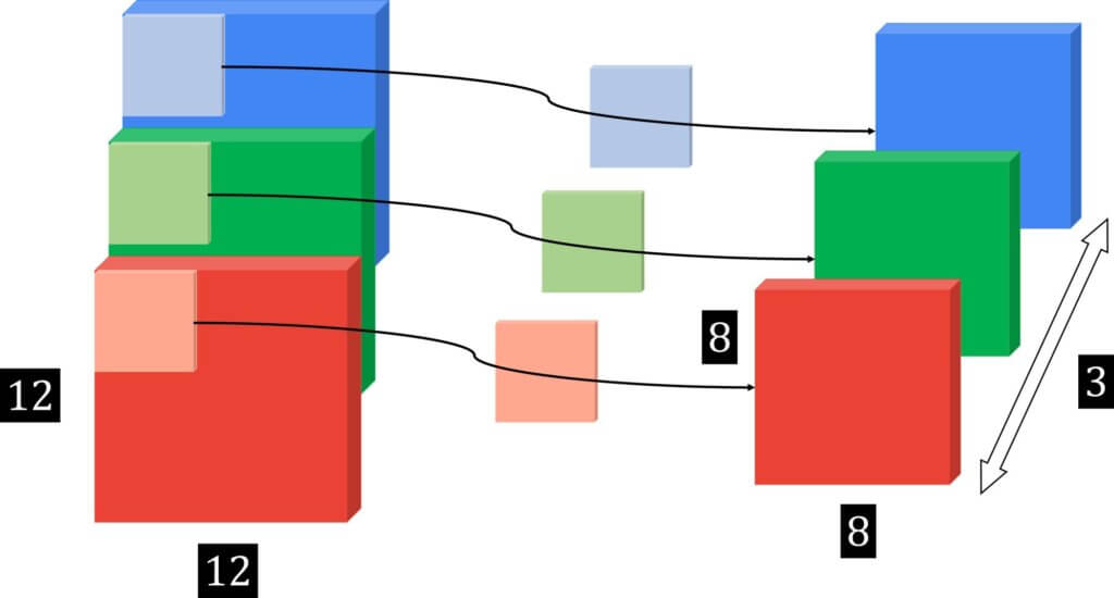
In addition, as far as the number of computations is concerned we will have:

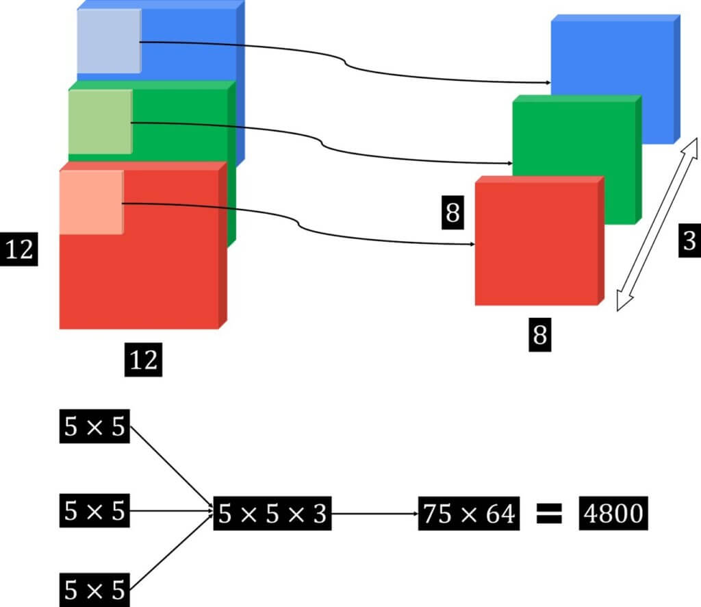
Subsequently, we will have to apply one additional step known as a point-wise convolution. Notice how it is calculated on the aforementioned obtained feature map of size \(8\times8 \).

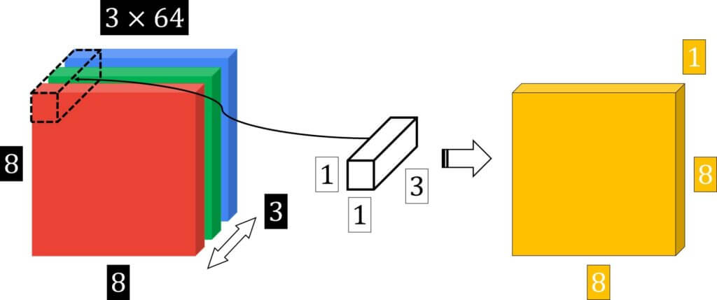
Without going too much into detail, we give credit to [1] and just compare that in this example:

depthwise separable convolution: 53, 952 operations
standard convolution required in total: 1, 228, 800 operation

Now, it makes it obvious why the use of depthwise separable convolution can be appealing.

2. The Encoder Part

We have already talked a lot about atrous (dilated) convolution in our previous post (DeepLab 002 link). You can check out our additional experiments to further understand this concept.

Here, we will just repeat that it is used within the concept of multiple rates that allows us to capture informative features for objects at different scales. In addition, one way to better describe the network is a simple term: output stride. This is the multiplicative ratio of how much the input image has shrunk after several blocks of the layer.

For instance, in image classification tasks, this factor is commonly 32. This means, that the input image size after convolutional layers (stride >1) and max-pooling layers is shrunk to a feature map with spatial dimension 32 times smaller.

In this DeepLab version, the output stride for the “feature extraction layers” is set to 16 (or 8). This is possible due to the use of atrous convolution. Finally, the feature map “before the logits” is used and passed further. That is, the final output activation function is removed and the feature map is passed to subsequent processing blocks.

Depth-wise Separable Convolution: The novelty in this work also represents the use of depth-wise separable convolution followed by a point-wise convolution (also known as \(1\times1 \) convolution). We have already explained and reviewed these two concepts.

Now, we will see how they are combined with the atrous convolution. “A picture is worth a thousand words” is true for the atrous depth-wise separable convolution. Have a look at the image below and you’ll know how easy it is to grasp the idea behind this convolutional based block:

Specifically, depth-wise convolution performs a spatial convolution independently for each input channel, and point-wise convolution is employed to combine the output from the depth-wise convolution.

Hence, the performance of the network is improved by the use of atrous depth-wise convolution that reduces the computational complexity. Note that in the block diagram, we still explicitly imply where the point-wise convolution is used, using the \(1\times1 \) convolutional block.

3. The Decoder Part

The decoder network starts with the output from the encoder part. In DeepLab v3, the output feature map is commonly downsampled 16 times as compared to the input image. In other words, the output stride for this block is 16. These features (just before the logit part in DeepLab v3), coming from the encoder, are first upsampled by a factor of 4 using bilinear interpolation.

As a refresher, we provide a simple example of applying bilinear interpolation in images.

The next step we will cite from the paper:

The encoder features are first bilinearly upsampled by a factor of 4 and then concatenated with the corresponding low-level features from the network backbone that have the same spatial resolution (e.g., Conv2
before striding in ResNet-101).

This sentence even raised a debate on the StackOverflow forum 🙂

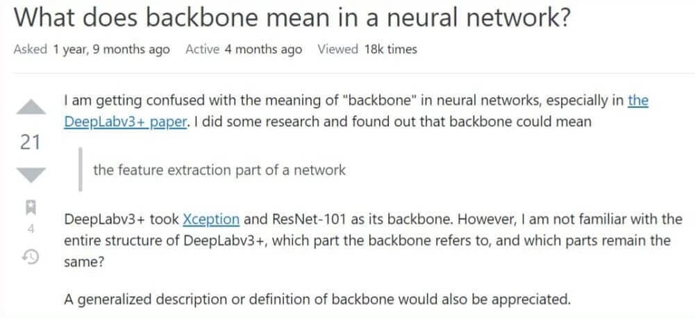
Here’s the answer we liked the best:

The backbone is used in DeepLab papers to refer to the feature extractor network. They are used to compute features from the input image. The authors have experimented with different networks such as MobileNet, ResNet, or Xception network. Herein, the following steps are applied as can also be seen in the image:

Apply \(1\times1 \) convolution to reduce the number of channels that are typically high: 256 or 512. This will make training easier.
Concatenate the features from the “backbone” and the encoder output.
Add few convolutional layers of kernel size \(3×3 \) to refine the features.
Perform bilinear upsampling by a factor of 4.
Get the final output containing the prediction.

We hope that we managed to convey the main ideas as proposed in the paper. Don’t worry if some of the details are still not clear. The main idea is to learn general concepts and ideas, especially, when and why to apply something. Even the authors experimented with a lot of different modules, changing them quickly through the iterative process.

You will gain more understanding from the PyTorch code that we will write next.

We will also get back to our term ‘backbone’. The initial part of the encoder can be based on the two choices:

ResNet-101 or
Xception Net

Modified Xception net when used as a backbone produces slightly better results.

Right! Let’s get straight into our code now.

4. Implementing DeepLab v3+ in PyTorch

Our code is inspired by the work presented in [2]. For full and complete code, you can refer to this work. In this post, we’ll just extract the most important modules necessary for code understanding.

First of all, we will start with the input and the layers that are first to process the image. We will have in total 5 layers that we use for processing and those are ResNet-101 layers which are trained on ImageNet.

After these five layers, the feature map is next passed to the ASPP module. It is implemented in DeepLab v3 network and the same version is used here.

After the ASPP, the feature maps are concatenated and are passed through the \(1\times1 \) convolutional filter.

 # Encoder 
ch = [64 * 2 ** p for p in range(6)] 
self.layer1 = _Stem(ch[0]) 
self.layer2 = _ResLayer(n_blocks[0], ch[0], ch[2], s[0], d[0]) 
self.layer3 = _ResLayer(n_blocks[1], ch[2], ch[3], s[1], d[1]) 
self.layer4 = _ResLayer(n_blocks[2], ch[3], ch[4], s[2], d[2]) 
self.layer5 = _ResLayer(n_blocks[3], ch[4], ch[5], s[3], d[3], multi_grids) 
self.aspp = _ASPP(ch[5], 256, atrous_rates) 
concat_ch = 256 * (len(atrous_rates) + 2) 

# here we have a 1x1 convolution where concatenated feature maps are passed    
self.add_module("fc1", _ConvBnReLU(concat_ch, 256, 1, 1, 0, 1)) 
Code language: PHP (php)

def forward(self, x): 
    h = self.layer1(x) 
    h = self.layer2(h) 
    # >> this feature "h_" is further passed to a decoder as a low level feature map
    h_ = self.reduce(h) 
    h = self.layer3(h) 
    h = self.layer4(h) 
    h = self.layer5(h) 
    h = self.aspp(h) 
    h = self.fc1(h) 
    h = F.interpolate(h, size=h_.shape[2:], mode="bilinear", align_corners=False) 
    # here we concatenate the 1) "low level feature map from encoder" and 
    # 2) the upsampled output of the encoder
    h = torch.cat((h, h_), dim=1) 
    h = self.fc2(h) 
    h = F.interpolate(h, size=x.shape[2:], mode="bilinear", align_corners=False) 
    return h 
Code language: PHP (php)

In the forward function, we concatenate variables “h_” and “h”. They are fed to fc2 module. This module is defined and in the decoder block since other parts are directly implemented in forward function (e.g. bilinear interpolation).

# Decoder 

    # this reduce is the 1x1 convolution applied on the low level feature map (h_)
    self.reduce = _ConvBnReLU(256, 48, 1, 1, 0, 1) 
    
    

    # here we process the concatenated the 1) "low level feature map from encoder" and 
    # 2) the upsampled output of the encoder

    self.fc2 = nn.Sequential( 
    OrderedDict( 
    [ 
    ("conv1", _ConvBnReLU(304, 256, 3, 1, 1, 1)), 
    ("conv2", _ConvBnReLU(256, 256, 3, 1, 1, 1)), 
    ("conv3", nn.Conv2d(256, n_classes, kernel_size=1)), 
    ] 
     ) 
    ) 
Code language: PHP (php)

Finally, we can include the ASPP block here as well, after the main flow of the algorithm is explained.

class _ASPP(nn.Module): 
    """ 
    Atrous spatial pyramid pooling with image-level feature 
    """ 
    
 
    def __init__(self, in_ch, out_ch, rates): 
        super(_ASPP, self).__init__() 
           self.stages = nn.Module() 
           self.stages.add_module("c0", _ConvBnReLU(in_ch, out_ch, 1, 1, 0, 1)) 
           for i, rate in enumerate(rates): 
               self.stages.add_module( 
                   "c{}".format(i + 1), 
                   _ConvBnReLU(in_ch, out_ch, 3, 1, padding=rate, dilation=rate), 
               ) 
           self.stages.add_module("imagepool", _ImagePool(in_ch, out_ch)) 
   
 
     def forward(self, x): 
           return torch.cat([stage(x) for stage in self.stages.children()], dim=1)

Atrous convolution is defined with the Conv2D function, where parameter rate defines dilation. It is interesting that the return from the ASPP module is the contatenated feature map from all atrous convolutions with different rates.

Semantic Segmentation in PyTorch Using DeepLab v3+

DeepLab v3+ was introduced in 2017 after several improvements
DeepLab v3+ combines atrous convolutions with multiple rates and the encoder-decoder structure using Xception Net architecture
Depth-wise separable convolution was used in DeepLab v3+ to reduce the number of operations
The feature extractor network is also known as the ‘backbone’ of the network, used to compute features from the input image in DeepLab v3+

Summary

That’s it friends! This post has come to an end. We hope we have managed to take you deep into the concept of DeepLab and semantic segmentation. Keep studying, revising and practicing the code by taking inspiration from the codes we present to you. You are a researcher-in-the-making and we wish you start writing your own models soon. Do send in your thoughts regarding this post or any feedback that you have for us. For more interesting content, follow us on Twitter and YouTube as well. We’ll see you next time with another interesting topic. Take care 🙂

References:

[1] https://www.youtube.com/watch?time_continue=1&v=vfCvmenkbZA&feature=emb_logo

[2] https://github.com/kazuto1011/deeplab-pytorch/blob/master/libs/models/deeplabv3plus.py

#023 PyTorch – DeepLab v3+ for Semantic Segmentation in PyTorch