#016 3D Face Modeling – Linear camera model

Highlight: In this post, we are going to talk about what calibration is and how it is performed. Calibration represents the process of going from one coordinate system to another, for example going from meters to pixels. We will explain how an image is formed, in more detail, how we go from the 3D scene in the real world to the 2D image plane in the camera.

In this post, we are going to review the YouTube video “Linear Camera Model | Camera Calibration”[1]. So let’s begin!

Forward Imaging Model: 3D to 2D

Let us start from the beginning, going from a 3D scene to a 2D image.

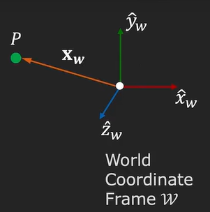
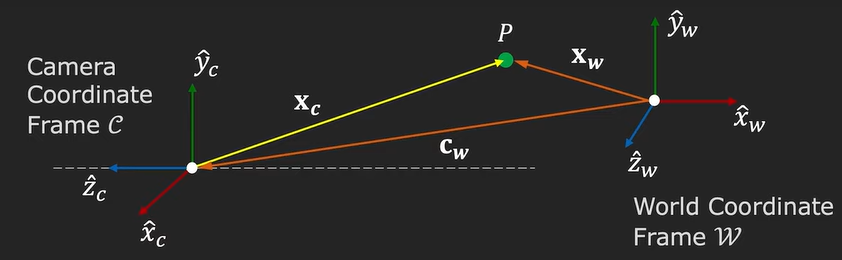
In the following image, we can see a world coordinate system, with 3 axes (\(x, y, z\)) and we have a point \(P\) that is located in this coordinate system.

Now, in this world coordinate frame lies a camera that has its own coordinate frame \(C\). The \(z\) axis of the camera coordinate frame is aligned with the optical axis of the camera. On the back of the camera, we will have an image plane where our 2D images will be projected on. The distance between the camera pinhole and the image plane is the so-called focal length, usually denoted as \(f\).

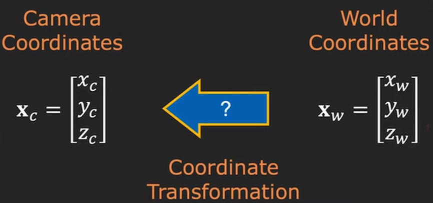
The goal is to go from this world coordinate system to the camera coordinate system. How can this be achieved?

By knowing the respective position of the camera to the world coordinate frame, an expression can be written that takes us from the point \(P\) in the world coordinate frame to its respective position on the image plane. And this process is what is usually called forward mapping.

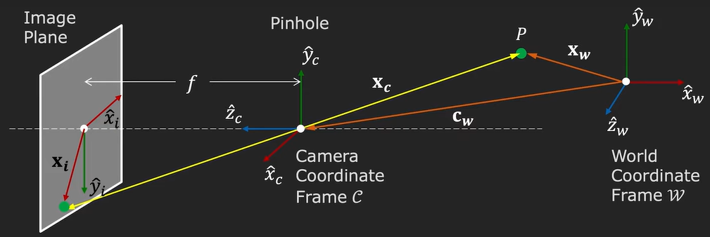
Let’s see how this is done. We first obtain the vector that is represented by the point \(P\), which we call \(x_w\). After this point, we transform the coordinates to the camera coordinates, \(x_c\) and we apply perspective projection to obtain image coordinates \(x_i\).

$$ x_i = \begin{bmatrix} x_i \\ y_i \end{bmatrix} \Longleftarrow x_c = \begin{bmatrix} x_c \\ y_c \\ z_c \end{bmatrix} \Longleftarrow x_w = \begin{bmatrix} x_w \\ y_w \\ z_w \end{bmatrix} $$

We have talked about perspective projection before (in this post), let us see now how it is derived and how we can calculate it for the camera. The projection takes the following form:

\(\frac{x_i}{f} = \frac{x_c}{z_c}\) and \(\frac{y_i}{f} = \frac{y_c}{z_c}\)

Or, it can be rewritten as: \(x_i = f\frac{x_c}{z_c}\) and \(y_i = f\frac{y_c}{z_c}\)

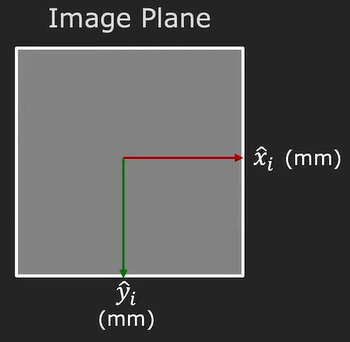
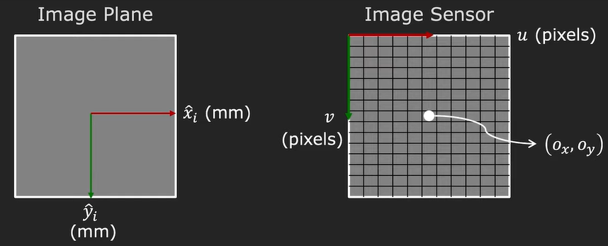
Moreover, we need to take into account the image plane. At the start, it is assumed that we know the coordinates of the image plane in millimeters which is the same unit where the point \(P\) is defined in the camera coordinate system.

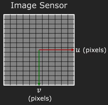
In reality, this will not be the case. Instead, we will have an image sensor that will capture the image. That sensor uses pixels as the main unit. We will have pixels that stretch in the \(x\) and \(y\) direction. So, we need to find a mapping from millimeters to pixels. These pixels are not always squares, as visualized below, they can also be rectangles.

To take into account all the shapes of pixels, we calculate the density of the pixels (pixels in a millimeter) in both \(x\) and \(y\) directions. To transform the unit from millimeters to pixels we just multiply these densities with the perspective projection equation.

$$ u = m_x m_i = m_x f \frac{x_c}{z_c}, v = m_y m_i = m_y f \frac{y_c}{z_c} $$

Also, one part that needs to be taken into account is the center of the image. By far we have assumed that it is at coordinates \((0, 0)\), where the optical axis pierces the image plane. This place is called the Principle Point. Usually, the top-left corner of the image sensor is treated as the image origin. This way we have eliminated negative coordinates for the image. The coordinates for the Principle Point are written as \(o_x, o_y\). If we shift the coordinates to the top left we need to add these values to the perspective projection equation. Then, we end up with a function that looks like the following:

$$ u = m_x f \frac{x_c}{z_c} + o_x, v = m_y f \frac{y_c}{z_c} + o_y $$

Because the \(m_x\) and \(m_y\) are unknowns, we can combine them with the focal length and this can be seen as the effective focal length. We end up with an equation:

$$ u = f_x \frac{x_c}{z_c} + o_x, v = f_y \frac{y_c}{z_c} + o_y $$

Looking at the formula above we can see two types of parameters, intrinsic and extrinsic parameters. The intrinsic parameters or the camera’s internal geometry are \(f_x, f_y, o_x, o_y\).

This equation now is not a Linear model, but rather a Non-Linear model. So, it is convenient to express them as linear equations. We will switch our coordinates from inhomogeneous to homogeneous and this way we are going from a Non-Linear model to a Linear one.

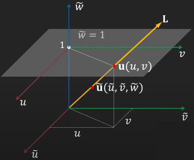
We have talked about this in a previous post, but just to remind ourselves how we can switch between these two coordinates. The homogeneous representation of a 2D point, \(u = (u, v)\) is a 3D point \(\tilde{u} = (\tilde{u}, \tilde{v}, \tilde{w})\). The third element that we added is called a fictitious coordinate or the equivalence class element.

Looking at the image below, we can define a \(u, v\) which is a plane where our point is located at.

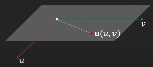
In relation to the plane, we can define a coordinate frame, \(\tilde{u}, \tilde{v}\), such that the previous \(u, v\) plane lies at \(\tilde{w}=1\).

To understand the homogeneous coordinates let’s take a look at an example. Looking at the image below, all the points that go from the origin (start of the yellow arrow), through the point \((u, v)\) and lie on this arrow, corresponding to homogeneous coordinates corresponding to the point \((u, v)\).

$$ u = \begin{bmatrix} u \\ v \\ 1 \end{bmatrix} = \begin{bmatrix} \tilde{w}u \\ \tilde{v}v \\ \tilde{w} \end{bmatrix} = \begin{bmatrix} \tilde{w} \\ \tilde{v} \\ \tilde{w} \end{bmatrix} = \tilde{u} $$

Now that we have seen how to represent points in homogeneous coordinates, let us transform our equations of the perspective projection, \(u = f_x \frac{x_c}{z_c} + o_x, v = f_y \frac{y_c}{z_c} + o_y \).

We can transform the \(u, v\) point into homogeneous coordinates:

$$ \begin{bmatrix} u \\ v \\ 1 \end{bmatrix} = \begin{bmatrix} \tilde{u} \\ \tilde{v} \\ \tilde{w} \end{bmatrix}$$

Taking the above equation of the perspective transformation and multiplying the left and right parts with \(z_c\) we get the following equation:

$$ \begin{bmatrix} z_c u \\ z_c v \\ z_c \end{bmatrix} = \begin{bmatrix} f_x x_c + z_c o_x \\ f_y y_c + z_c o_y \\ z_c \end{bmatrix} $$

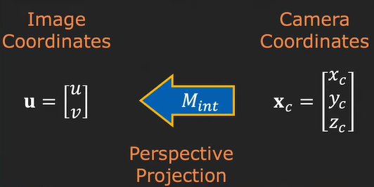
This equation can be further simplified, by placing everything in matrices. One \(3\times4\) matrix that includes all the internal parameters of the camera multiplied by the matrix with homogeneous coordinates of the 3D point defined in the camera coordinate frame. These steps give us a linear model for perspective projection and it is called the intrinsic matrix.

$$ \begin{bmatrix} u \\ v \\ 1 \end{bmatrix} = \begin{bmatrix} \tilde{u} \\ \tilde{v} \\ \tilde{w} \end{bmatrix} = \begin{bmatrix} f_x & 0 & o_x & 0 \\ 0 & f_y & o_y & 0 \\ 0 & 0 & 1 & 0 \end{bmatrix} \begin{bmatrix} x_c \\ y_c \\ z_c \\ 1 \end{bmatrix}$$

Now we have now seen how we can go from the camera coordinates to the image coordinates using perspective projection and we have seen how to get a linear model.

The next important step is going from world coordinates to camera coordinates. This step can be done by using the position and orientation of the camera coordinate frame with respect to the world coordinate frame.

The position is given by a vector \(c_w\) and the orientation is given by a matrix \(R\). This matrix is a so-called rotation matrix, which is \(3\times3\). How can we describe this matrix?

The first row is the direction of the vector \(\hat{x}_c\) in the world coordinate system. The second row is the direction of \(\hat{y}_c\) and the third is the direction of \(\hat{z}_c\). Also, note that the rotation matrix is an orthonormal matrix.

This rotation matrix \(R\) and the distance vector \(c_w\) represent the extrinsic parameters of the camera. We can take the point \(P\) and we want to convert it to the camera coordinate system. We take the vector \(x_w\) from the world coordinate frame and subtract the \(c_w\) (the distance between the origin of the world and camera coordinate systems). This value that we get we will multiply this with the rotation matrix and as the result, we obtain the point \(P\) in the camera coordinate frame.

$$ x_c = R (x_w – c_w) = Rx_w – Rc_w = Rx_w + t, t = -Rc_w$$

To write this in matrix format, we separate the matrix into the rotation and translation parts. Then we multiply the rotation with the world coordinates and just add the translation vector.

$$ x_c = \begin{bmatrix} x_c \\ y_c \\ z_c \end{bmatrix} = \begin{bmatrix} r_{11} & r_{12} & r_{13} \\ r_{21} & r_{22} & r_{23} \\ r_{31} & r_{32} & r_{33} \end{bmatrix} \begin{bmatrix} x_w \\ y_w \\ z_w \end{bmatrix} + \begin{bmatrix} t_x \\ t_y \\ t_z \end{bmatrix} $$

To write everything compactly into one matrix, we can move these systems to homogeneous coordinates and add the translation vector next to the rotation matrix.

$$ x_c = \begin{bmatrix} x_c \\ y_c \\ z_c \\ 1 \end{bmatrix} = \begin{bmatrix} r_{11} & r_{12} & r_{13} & t_x \\ r_{21} & r_{22} & r_{23} & t_y \\ r_{31} & r_{32} & r_{33} & t_z \\ 0 & 0 & 0 & 1\end{bmatrix} \begin{bmatrix} x_w \\ y_w \\ z_w \\ 1 \end{bmatrix}$$

Now we have two types of matrices, intrinsic and extrinsic matrices. The intrinsic matrix is represented as \(M_{int}\) and the extrinsic as \(M_{ext}\). So, we first go from world coordinates to the camera, and then from camera coordinates to pixels on the image plane (from millimeters to pixels).

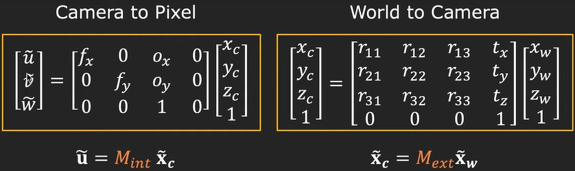
All of this can be combined as the product of \(M_{int}\) and \(M_{ext}\) which is a single matrix \(P\), which is a \(3\times4\) matrix called the projection matrix.

$$ \tilde{u} = M_{int}M_{ext}\tilde{x}_w = P \tilde{x}_w $$

$$ \begin{bmatrix} \tilde{u} \\ \tilde{v} \\ \tilde{w} \end{bmatrix} = \begin{bmatrix} p_{11} & p_{12} & p_{13} & p_{14} \\ p_{21} & p_{22} & p_{23} & p_{24} \\ p_{31} & p_{32} & p_{33} & p_{34} \end{bmatrix} \begin{bmatrix} x_w \\ y_w \\ z_w \\ 1 \end{bmatrix} $$

Summary

In this post, we have seen what the intrinsic and extrinsic parameters are and what they look like. This is important for the calibration process because if we want to calibrate a camera we just need to know this projection matrix or we need to know the 12 numbers from the projection matrix and we can go from any point in the 3D world coordinate system to the image plane.

References:

[1] – Linear Camera Model | Camera Calibration – Shree Nayar, T. C. Chang Professor of Computer Science in the School of Engineering at Columbia University