Highlight: This post can come as a very interesting and surprising one. You will see how we can apply a machine learning algorithm on the pixel intensity color with a so-called K-means clustering algorithm. In this way, we would be able to create a compressed version of our image that will have much fewer colors. The picture will be preserved in a lower color resolution, whereas the number of pixels will remain the same. This technique is very exciting, so we hope that you will enjoy it.

Tutorial Overview:

1. What is K-Means algorithm?
2. Color quantization with K-Means algorithm
3. Experiments in Python and OpenCV

1. What is K-Means algorithm?

K-Means represents an unsupervised algorithm from machine learning theory. This algorithm aims to cluster input data points and is one of the most straightforward and intuitive clustering algorithms, among many others. The input data points need to be assigned to different clusters based on the similarity between them. The easiest way to measure the similarity between different objects/data points is to calculate the distance between them. The most commonly used measure of a distance between two points is the Euclidean distance. We are very much familiar with the distance between two cities or points in a 2D plane.

We will explain the K-Means algorithm using a dataset that can be represented in a 2D plane. As input, we will have a certain number of points. Before we start executing K-Means, we need to specify how many clusters we want, i.e., set a value of K. However, finding an optimal number of clusters is not an easy task sometimes.

There are some particular methods that can be utilized and experimented with to find an optimal number of clusters, as this is not an easy task sometimes. For instance, if you would like to cluster books in a library, you will not know in advance how many labels you need to use. In a library, you can have computer vision books in one section and maybe machine learning books in another one. On the other hand, you can create three clusters with computer vision, image processing and machine learning books depending on the number of books from each category. You get the idea.

The basic definition of the K-Means algorithm can be separated into two parts. The first part is the cluster assignment step in which we will randomly choose K points in our 2D plane as cluster centers. Then, we will loop over all input data points one by one and  assign the closest cluster center to each data point based on some distance measure, e.g., Euclidean distance. In this way, we will make each data point a member of the nearest particular cluster.

After this, we will have a second step, i.e., updating the cluster centroids. As the initially randomized K centers are not a true representative of the clusters, , hence, we will find new or updated centers by changing the existing centroids. For this purpose, we will use the following formula as given below:

$$ m_{i}^{(t+1)}=\frac{1}{\left|S_{i}^{(t)}\right|} \sum_{x_{j} \in S_{i}^{(t)}} x_{j} $$

This formula will give us mean values for \(x \) and \(y \) coordinates over all data points in a cluster. We will take these mean values as the new coordinates for each cluster centroid. Hence, using these updated centers, we will have an updated situation regarding different data points. It may happen that due to changing in the cluster centroids, some data points lying in the borderlines between two clusters will now have to be reassigned.For example, if a center has moved away point during the update, there is a chance that the data points initially lying at the border of that specific cluster will have to be reassigned to some another centroid.

The above two steps will be edit relatively until the algorithm converge once there is no further change in cluster centroids in two successive iterations. At this stage, there will be no more changes in clusters assignment and there will be no further update step. Once we assign color with this method, here color=km.labels_, every data point will be colored according to the label where it belongs to. You can see an example of K-Means algorithm in the following GIF animation.

So, the best way to understand K-Means is actually to use the code.

Once we start with K-Means, first thing that we need to do is to generate our data samples or points. One easy way of doing this is to use make_blobs()function from sklearn. It is very intuitive to use this function and as an input, we just provide the number of samples (100 in the code sample given below) and number of features(i.e., the dimension of the data point). If we have a 2D plane, it means that we will have the number of features equals to 2).

# Necessary imports
import numpy as np
from sklearn.cluster import KMeans
import cv2
import matplotlib.pyplot as plt
from sklearn.datasets import make_blobs
from google.colab.patches import cv2_imshow

X, y = make_blobs(n_samples = 100, n_features=2, centers = 4)

Although for this example, we specify that we have just four blobs; however, our K-Means algorithm does not know that in practice.  We can experiment with K equals to 2 or 3, or 4, and so on. To see what the result looks like since this is just an introductory example, we will assume that indeed we have 4 points and we will cheat a little bit to make this first introduction of K-Means algorithm a little bit easier.

In this case, we will use K-Means algorithm implemented in sklearin library. As you can see, we will create our \(X \) point, and we also have a variable \(y \) that tells us from which cluster does a particular point comes from. But in practice, once we work with K-Means, we will forget that we actually have this variable.

After plotting our points with function plt.scatter(), we will get the image that looks like this.

# Plotting our points with plt.scatter
plt.scatter(X[y==0,0], X[y==0,1])
plt.scatter(X[y==1,0], X[y==1,1], c='r')
plt.scatter(X[y==2,0], X[y==2, 1], c='b')
plt.scatter(X[y==3,0], X[y==3, 1], c='g')

Output:

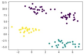
With the following functions, we can generate our output very quickly. The output of the K-Means algorithm will be the so-called labels. These labels represent our prediction of the algorithm that tells which data points will be assigned to what clusters. By accessing the km.labels variable, we can print these labels to get an idea where these clusters data points belong to.

# n_clusters = 3, 
km = KMeans(n_clusters=3)
km.fit(X)
y_km = km.predict(X)

# Printing labels by accessing the km.labels variable
print(km.labels_)

Output:

[2 0 2 2 1 0 0 1 0 1 0 0 0 1 1 0 0 2 2 0 2 0 0 0 0 1 1 1 2 2 1 0 0 0 2 0 2 0 2 0 1 0 0 0 1 0 2 1 1 1 1 0 0 1 2 0 0 0 0 0 0 0 0 0 2 1 1 0 0 1 2 0 0 2 1 0 1 2 0 0 0 1 2 0 2 2 1 2 0 2 0 2 1 1 0 2 2 0 0 0]

# We can see how we can use this vector for the graphic illustration
plt.scatter(X[:,0], X[:,1], c=km.labels_, cmap='viridis')

Output:

# Defining the cluster centers
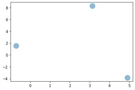
plt.scatter (km.cluster_centers_[:,0], km.cluster_centers_[:,1], s = 200, alpha = 0.5)

Output:

plt.scatter(X[:,0], X[:,1], c=km.labels_, cmap='viridis')
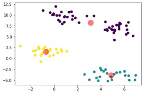
plt.scatter (km.cluster_centers_[:,0], km.cluster_centers_[:,1], s = 200, alpha = 0.5, c='r')

Output:

 2. Color quantization with K-Means algorithm

Now, we come to the second part, where we will explain what color quantization actually means. One way of comparing two colors is to calculate Euclidean distance between them, which will be done with the following formula:

$$ \sqrt{\left(R_{1}-R_{2}\right)^{2}+\left(G_{1}-C_{2}\right)^{2}+\left(B_{1}-B_{2}\right)^{2}} $$

So, here we see that every pixel is defined with red, green, and blue. For two data points, we will just make these subtractions. The closer these points are in this 3D color space or a cube, the lower the Euclidean distance will be. In the case where we have very distant colors, this Euclidean distance will be relatively larger. For instance, white and black will be very far apart. On the other hand, any certain two points will be relatively close. We can better understand this if we look at the following example:

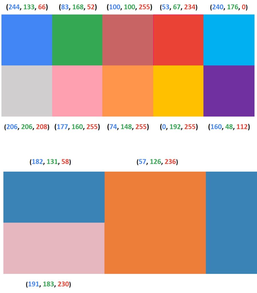
In this example, we can see our original image where each square represents a single color pixel. We can also see the values of these pixels represented in RGB order. We applied color quantization with K-Means algorithm on the original image and obtained our quantized image with only 3 colors. (Note that pixel values in the output image are represented in BGR order).

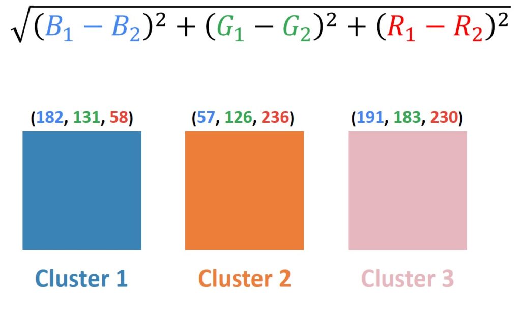
Now we can calculate Euclidean distance between these colors and several other pixels from our input image

You can see in our examples that after calculating Euclidean distance, we obtained 3 results for each cluster. The lowest Euclidean distance value determines that two points are closest to each other (e.g., 53.72 is the lowest value in the first example, 162.21 is the lowest value in the second example and 101.43 is the lowest value in the third example).

Now, we will experiment a little bit with Python code, were we are going to use OpenCV function cv2.kmaeans(). This function implements a K-Means algorithm, which finds centers of clusters and groups input data points around them. In the following picture, you can see the parameters that are implemented in this function:

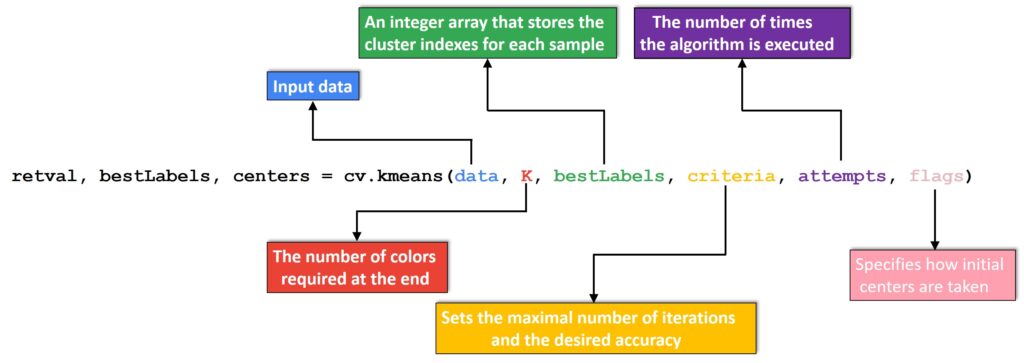
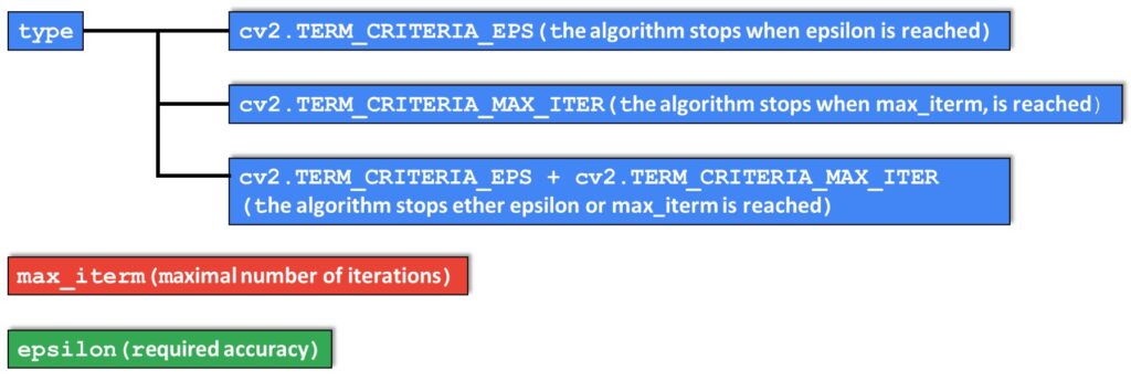
The parameter data represents the input data for clustering. Note that it should be of np.float32 data type. K specifies the number of clusters (colors) required at the end. You can see the criteria parameter in the following example, which sets the maximal number of iterations and the desired accuracy.

3. Experiments in Python and OpenCV

Now we can run our code. Our goal is to reduce the number of colors in the original image by using the K-means clustering algorithm for displaying output with a limited number of colors. We will perform color quantization using a few different values for K. Let’s look at our results.

# Loading our image
img = cv2.imread('beach.jpg',1)
cv2_imshow(img)

Output:

def color_quantization(img, k):
# Defining input data for clustering
  data = np.float32(image).reshape((-1, 3))
# Defining criteria
  criteria = (cv2.TERM_CRITERIA_EPS + cv2.TERM_CRITERIA_MAX_ITER, 20, 1.0)
# Applying cv2.kmeans function
  ret, label, center = cv2.kmeans(data, K, None, criteria, 10, cv2.KMEANS_RANDOM_CENTERS)
  center = np.uint8(center)
  result = center[label.flatten()]
  result = result.reshape(img.shape)
  return result

# Applying color quantization with different values for K
color_3 = color_quantization(img, 3)
cv2_imshow(color_3)
color_8 = color_quantization(img, 8)
cv2_imshow(color_3)
color_13 = color_quantization(img, 13)
cv2_imshow(color_3)
color_20 = color_quantization(img, 20)
cv2_imshow(color_3)
color_40 = color_quantization(img, 40)
cv2_imshow(color_3)

Now we can look at our results.

Output:

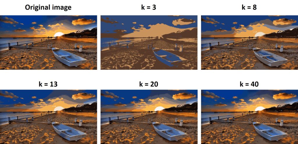
Amazing, right? The second example is probably the most fascinating. We managed to reduce the number of colors to only 3 while preserving the overall appearance quality.

Summary

In this post, we learned what K-means clustering algorithm is and how to apply color quantization on images using this algorithm. We showed how we can create a compressed version of our image with a fewer number of colors using the K-means algorithm. In the next post we will explain how to detect faces, eyes and smiles using Haar Cascade Classifiers.

References:

[1] Mastering OpenCV 4 with Python by Alberto Fernández Villán