#005 GANs – Face editing with Generative Adversarial Networks
Highlight: Over the past few years in machine learning we’ve seen dramatic progress in the field of generative models. While there are a lot of different flavors of these generative models in this post we want to talk specifically about one model called the Generative Adversarial Network or in short GAN. Have you ever wanted to see what you would look like as part of the opposite gender? Or what about playing with the age of Barack Obama or making Emilia Clark smile. Well in this post we will show you how to play with a latent space of the most powerful generative models that we have available today. And everything we’ll be doing in this post you can do for yourself on any image that you want. Are you ready to dive in deep? Let’s start.
Tutorial Overview:
- Introduction to GANs
- Arhitecture of GANs
- GAN objective functions
- State-of-the-art GAN techniques
- How to use the latent space to manipulate any image that you want?
1. Introduction to GANs
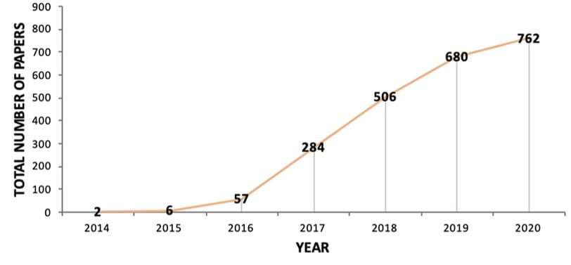
Now GANs were first invented by Ian Goodfellow in 2014 [1]. Since then these models have seen an incredible burst of research improvements and applications. The following graph shows the cumulative number of publications related to GANs per year. As you can see the number of papers was only 2 in 2014, and then, it skyrocketed in recent years [2].
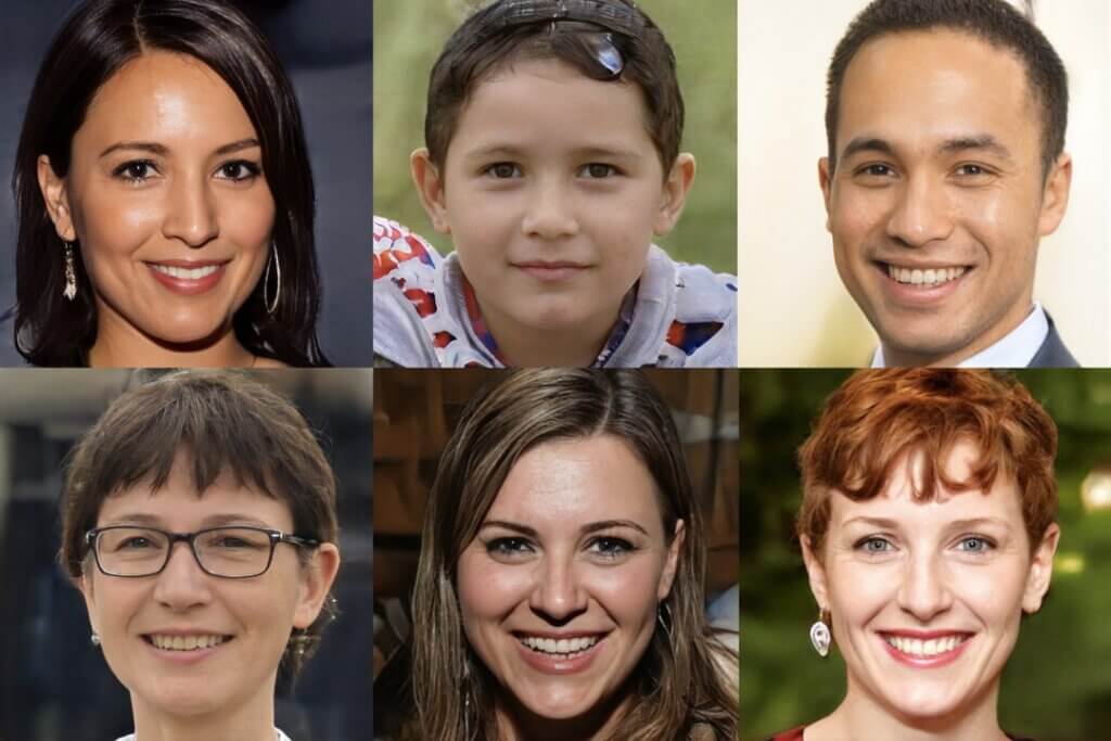
One of the coolest things about GANs is that we can take the underlying architecture, and then, we can train the model on any dataset that we want. So, most famously the researchers at Nvidia have trained these models to generate faces leading to the popular website ThisPersonDoesNotExist.com. In the image below you can see the several fake faces that are generated by the GANs.
We can take the same underlying model and we can train this on anything that we want. For example, we could train it on cats or on cars or bedrooms. Basically, anything you have in terms of an image data set you can use to train this generative model. And because most of these generative models are open-sourced by their creators, a lot of nifty people on the internet have trained their own models on a variety of data sets. Needless to say, training your own generative model can be a lot of fun. But that’s not everything. It turns out that when you train a generative model on a data set, which is, by the way, a fully unsupervised process because you’re not using any labels, it turns out that these models actually discover the underlying structure in that data set. And once the model has discovered this structure you can actually start using and exploiting that to do a variety of pretty cool things. So in this post, we want to give you an overview of what you can actually do with the latent space of a generative model once it has been trained on a particular data set.
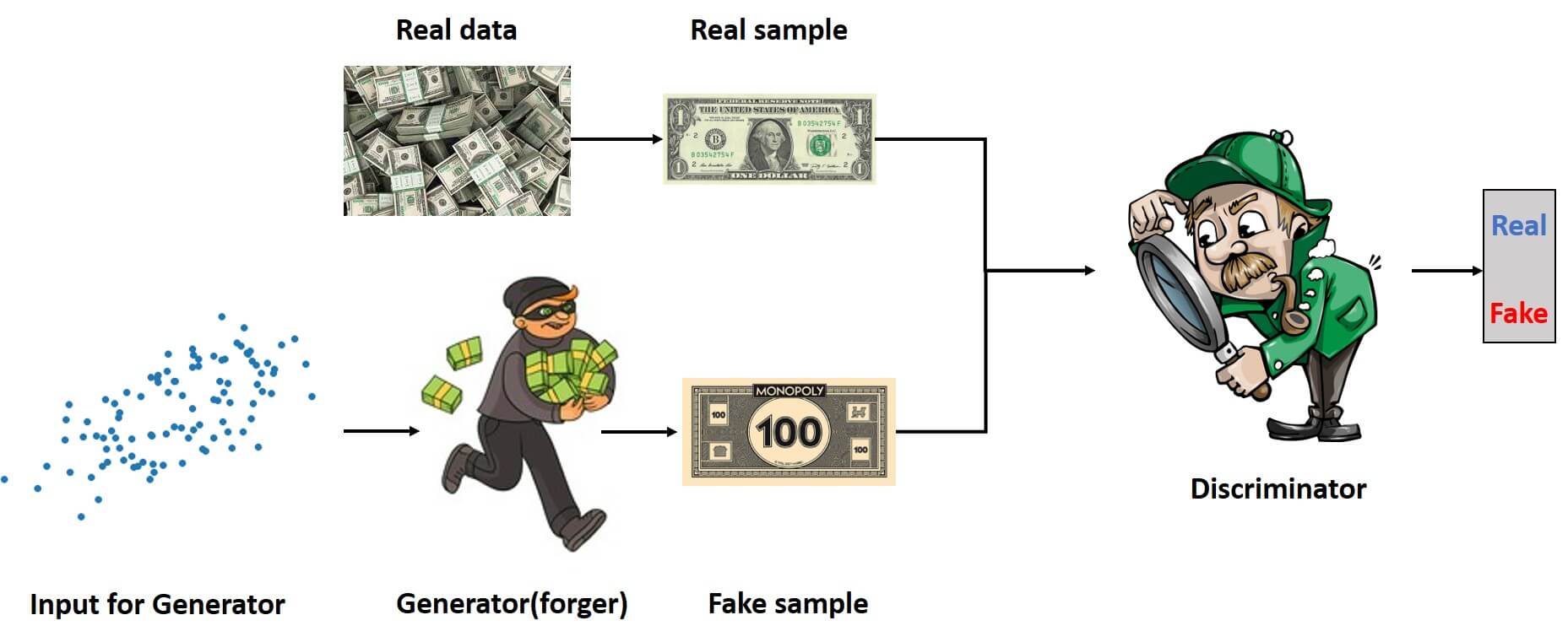
Before, we proceed, let’s introduce the GAN theory in an intuitive way. If you watched the movie “Katch me if you can” you remember the character of a skilled forger Frank Abegnale Jr played by Leonardo DiCaprio. The second character is the police inspector Carl Hanratty played by Tom Hanks. These two characters are adversaries. Leonardo DiCaprio throughout the movie is trying to deceive a police officer, while the police officer tries to catch him in his fraudulent activity.
The idea behind GANs is similar to the relationship between Leonardo DiCaprio and Tom Hanks in the movie. It is a simple but also very beautiful idea. We have two neural networks that are adversaries. They constantly fight with each other and they behave similarly to the forger and policeman. This process is illustrated in the following image.

Now, let’s have a look at the architecture of the GANs in more detail.
2. Arhitecture of GANs
So, let’s say that we are want to build the network that generates the image of a face. The first thing that we need is the training dataset that consists of the real images of human faces. Then we have two networks called generator and discriminator.
Generator
The first network is called a generator. This network is a forger. It gets a randomly sampled noise vector as an input. In most cases, it is a sample from a Gaussian distribution. Then we follow through with plenty of convolutional layers and at the end, the network generates an image as an output.
Discriminator
The second neural network is called the discriminator. It is a standard supervised learning classifier. As an input, it takes fake images from the generator and the real images from the actual training dataset. The discriminator has one job. It needs to decide whether that image is real or fake.
The architecture of the GANs is illustrated in the image below.
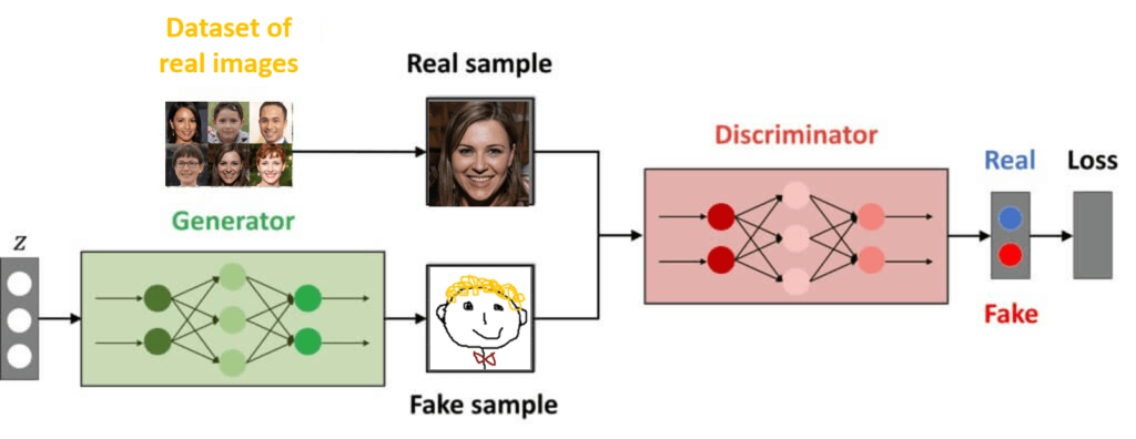
The important thing to remember is that the images from the data set are not labeled. However, for each image that we feed to the discriminator, we know whether that image is coming from the dataset or it is an image from the generator. By using this label we can basically backpropagate a training loss through this discriminator network in order to make it better.
Another interesting thing is that this generator network itself is also a fully differentiable neural network. So, if we stick together these two networks, we can actually backpropagate the learning signal through this entire model pipeline. In this way, we can update with the same single loss function both the discriminator and the generator network until they both get really good at their job.
The most important trick in this pipeline is to make sure that both these networks are well balanced during training. In that way, no one of them gets the upper hand. However, if we train the network for a long time, we will end up with a generator that has been learning from the feedback of the discriminator network. Then, eventually, it will be able to generate images that look very similar to the real images from the dataset we’ve been training on.
3. GAN objective functions
Now, let’s do a technical deep dive on the objective function that is used while training. So we are going to look at the original objective function as it was published in Goodfellow’s paper in 2014. Basically what’s happening is that the generator and the discriminator are playing a minimax game. Let’s explain this game in a little bit more detail.
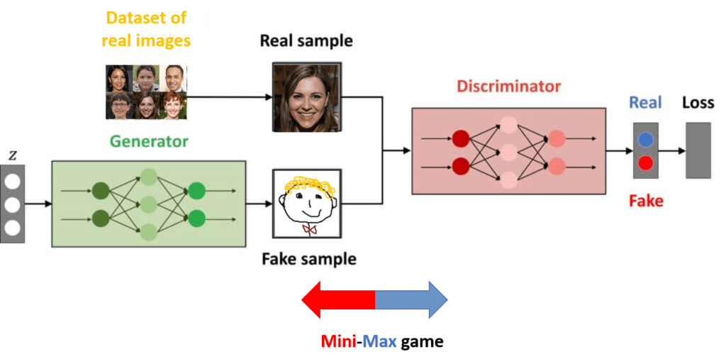
The generator is trying to create images that actually fool the discriminator and the discriminator is always trying to be right. In that game that they are playing with each other, they try to exploit the weaknesses of their adversary. In that process, they are forcest to fix those weaknesses in themself because their opponent is also exploiting their weaknesses. So, every time the network finds a strategy that works very well against their opponent, the opponent needs to find a way to deal with that strategy. In other words, as the system gets better it forces itself to get better because it continuously plays a game against a better opponent. This game between generator and discriminator is the minimax game and can be described with the following equation.
$$ \min _{G} \max _{D} \mathbb{E}_{x \sim q_{\text {data }}(\boldsymbol{x})}[\log D(\boldsymbol{x})]+\mathbb{E}_{\boldsymbol{z} \sim p(\boldsymbol{z})}[\log (1-D(G(\boldsymbol{z})))] $$
This equation is divided into two parts. The first part of the equation describes the discriminator. So, the discriminator network takes the real image as an input and outputs a single scalar value \(D(x) \) between 0 and 1. This value indicates how likely it is that this image \(x \) is a real picture of a face that comes from the dataset. If the output is equal to 1 then it is the real image and if the output is equal to 0 it is the fake image.

For generated images \(G(z) \) where \(z \) is the noise vector, the network outputs a score \(D(G(z)) \) of these fake images. Again, if the output is equal to 1 then it is the real image, and if the output is equal to 0 it is the fake image.

Our goal is that the discriminator recognizes the images \(x \) from the dataset as real images. So, for output, we want a high value close to one. At the same time, we also want the discriminator to recognize the generated images \(G(z) \) as fake. Therefore, we want the output value to be close to zero.
Then, the two networks are trained simultaneously. In particular, the objective is optimized as a minimax optimization problem that is solved using alternate optimization until convergence is reached. The important thing to remember is that here we do not have a human to perform the labeling. Class 0 simply means that the image is created from a generator, whereas class 1 is assigned to every true image from the original dataset.
Now let’s explain the training process in a little bit more detail. So, at every training step of the algorithm, we’ll start with two things. We sample a batch of random noise vectors and a batch of images from the data set. Then, we’re going to freeze the generator network and use the objective function in order to update the parameters of the discriminator to calculate the loss. Recall that the discriminator should output a value of 1 or close to 1 in case the image is real. Hence, the term \(log(D(x)) \) should be maximized.
$$ log(D(x))\to max $$
This is due to the fact that the \(log() \) function is monotonically increasing. So, to maximize \(log(D(x)) \) we need to maximize \(D(x) \). This will be done by setting \(D(x) \) as close as possible to 1 since the output of \(D(x) \) is limited to the interval [0, 1].
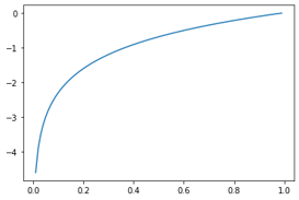
We also want to maximize the second term of the equation. That means that \(log(1- D(G(z))) \) should be as large as possible. Obviously, this will be achieved by setting a term \(D(G(z)) \) as close as possible to zero. This makes perfect sense since we want a discriminator to classify all generated images as fake (class 0). In the equation, this is denoted with the operator for mathematical expectation where the \(z \) vector is distributed over \(p(z) \). In other words, for all images that are generated with a set of vectors that follows \(p(z) \) distribution, we want to get \(D(G(z))=0 \) or as close as possible to zero. This would be the behavior of a nicely trained discriminator \(D \). Note, that while we are training a discriminator network, the parameters of the generator will be fixed and treated as constants.
Finally, after calculating the loss we will apply a gradient ascent algorithm to update the parameters.
Once we’ve updated the discriminator, then we freeze the weights of the discriminator and we go to another part where we actually train the generator.
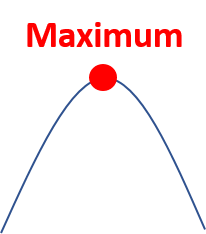
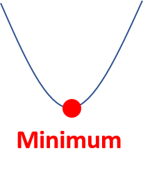
Here, we want an objective function to be maximized so that we can get a perfect discriminator. However, the goal of the generator is to fool the discriminator as much as it can. Hence, it will try to do the opposite which is to minimize the objective function.
$$ log(D(G(z)))\to min $$
In practice, this means that the term \(log(1-log(D(G(z))) \) is as small as possible. This makes sense, as we want a discriminator to be fooled. That is, the term \(D(G(z)) \) we want to be as close as possible to 1. In this way, the term \(log(1-log(D(G(z))) \) will actually be minimized, which is the goal of the generator.
After training the generator, we will then apply the gradient descent algorithm on that second part of the objective function in order to update the parameters of the generator.
If we then put this objective function into a concrete algorithm this is what we get:
$$ \nabla_{\theta_{d}} \frac{1}{m} \sum_{i=1}^{m}\left[\log D\left(\boldsymbol{x}^{(i)}\right)+\log \left(1-D\left(G\left(\boldsymbol{z}^{(i)}\right)\right)\right)\right] $$
So, this is the whole algorithm. In practice, there are a few additional tricks that you can apply to make sure that this objective function actually converges nicely and smoothly because it tends to be a little bit unstable in the exact form that we’ve just seen. Nowadays we have a wide variety of objective functions that people use to train GANs but all of them are built on the same core idea that we just saw in the algorithm.
4. State-of-the-art GAN techniques
So before we start actually messing around with some real images let’s first introduce two final ideas that we’re going to be using in our generative model. The first one is the progressive growth of the layers in your generative model. This was an idea published by Nvidia in their paper called “Progressive Growing of GANs”.
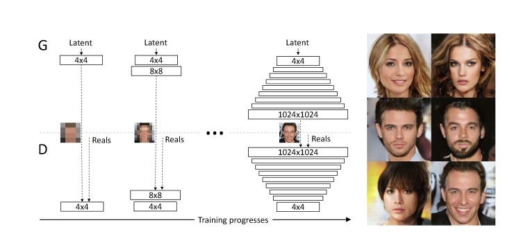
The idea here is in fact not that difficult either. As you can see in the image above we basically start with a generative model that generates very very small images of super-low resolution and at the same time the discriminator also gets to discriminate between very low-resolution images. This makes the entire process actually super simple so this network is very stable and it converges quickly. Once that network has stabilized you then simply add an additional layer to both the generator and the discriminator architecture which works at a slightly higher resolution and you keep on training.
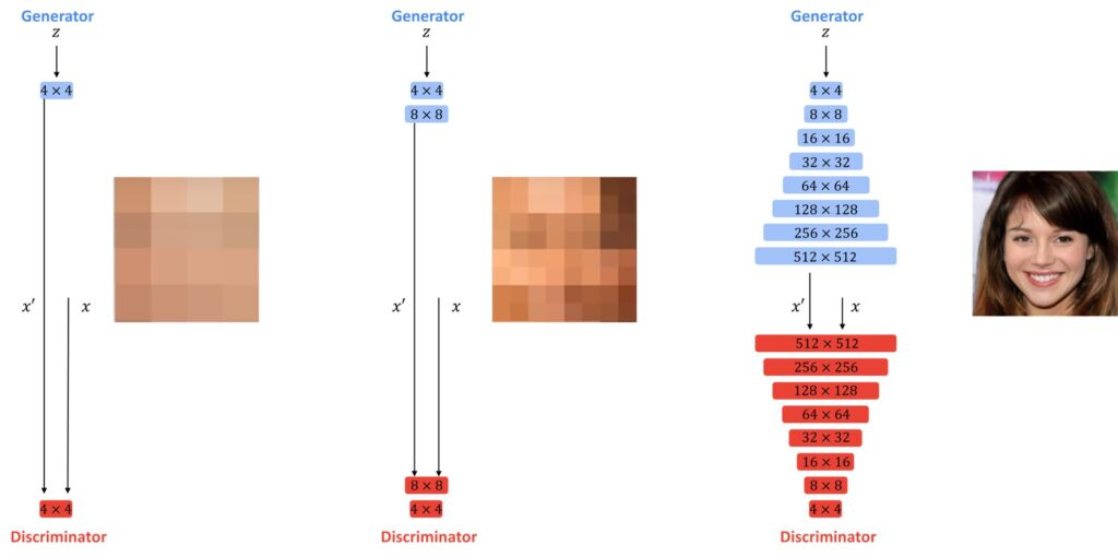
There are a few additional tricks where instead of just adding this one layer, we basically do it gradually by blending the previous layer towards the higher resolution. In practice, this is what happens. Your generator starts by generating very low-resolution images and the discriminator discriminates them. Then during the training process, you gradually scale up the resolution of the images in your training pipeline.
The second very influential paper by Nvidia in the generative model landscape was a model architecture called StyleGAN. In fact, StyleGAN is the model that we’re going to be using to manipulate our images. So traditionally what happens is that you take a generator architecture and it gets a random noise sample as an input. You feed that noise sample through a whole bunch of upsampling and convolutional layers until you get an image. What the style gain generator does is slightly different.
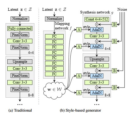
First, it has a mapping network. This mapping network takes the noise vector \(z \) and transforms it into a different vector called \(w \). The important thing here is that the \(w \) vector doesn’t have to be Gaussian anymore. The distribution of those \(w \) vectors can be whatever the generator wants it to be. Then the actual generator architecture doesn’t start from a random noise vector anymore it starts from a constant vector. This constant vector is actually optimized during training. So it’s kind of like a fixed seed in the beginning of the first layer of the generator architecture but the actual numbers of that seed, the values of that vector, are constant but they’re optimized during the training process. Finally the output of the mapping layer \(w \) is plugged into multiple layers of the generative architecture using a blending layer called AdalN. And during training also add noise to these parameters.
If you wondering why you would use a mapping layer like this, here is the answer.
Imagine that you have a data set. Then imagine we look at two properties: gender and facial hair. So we have male and female and we have a beard and no beard. Well in most image datasets of people you will find very few women that have beards. In other words, our data distribution has a gap there. And if we’re sampling from a Gaussian distribution, that distribution is uniform so it doesn’t have any gaps. So this is essentially what this mapping network allows you to do. It allows you to sample from a uniform distribution but then warp that distribution in such a way that you can have gaps for example where there are no actual images. And the idea is that if this warping of the space is already done by the mapping network (your \(w \) vector is already in a good shape) then your actual generator who takes that vector and turns it into an image has a much simpler job of doing that. Because the relationship between images and the input vectors is more one-to-one. It doesn’t have any gaps or strange distortions that it has to learn.
That is the Style GAN generator architecture. In the Style GAN paper, they apply this generative architecture you know which starts from a constant and uses a mapping layer, but they also use the progressively growing of the layers. With those two tricks combined, they were able to create a very powerful GAN that was able to produce incredibly realistic images.
4. How to use the latent space to manipulate any image that you want?
The general principle that we’re gonna leverage here is that when you train a generative model the latent space usually learns the underlying structure of your data set. Again that structure is learned fully unsupervised by the generative model because we’re not using any labels in the data set. So how can we leverage this structure? The core idea is that instead of manipulating images in the pixel domain, which is really difficult and very complicated, we’re gonna manipulate images in the latent space of that generative model. In order to do this starting from any given image, we’re gonna have to find a way to find a query image inside the latent space of the generator. More specifically let’s say that we start with this image of Michael Jordan. The question is well how can we find the latent vector \(z \) such that if we send \(z \) through the generator we get this image of Michael Jordan.
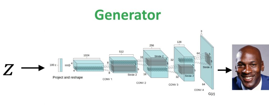
That’s the first problem we’re gonna have to solve. You could try randomly sampling a whole bunch of these latent vectors and see which one is closest but that’s gonna take a really long time. We’re gonna need a better approach. So one of the most straightforward things that you could try is that, given the fact that this generative model is a fully differentiable neural network, you can send gradients through it. You could basically randomly start from any latent vector \(z \). You generate a random image but then you compare that image to the query image of Michael Jordan. And you could define a simple loss function let’s say the pixel by pixel difference ( \(L2 \) difference between these two images ) and you can do gradient descent. Not on the image but you send your gradients through this generator model and you actually update the latent vector \(z \) at the beginning of your generator.
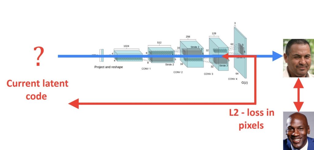
So by applying gradient descent on this \(L2 \) pixel loss we could in theory find the optimal latent vector \(z \) that gives us a good image of Michael Jordan. Unfortunately, this doesn’t really work. The \(L2 \) optimization objective is going to start going in the direction of Michael Jordan but before it gets there it’s gonna get stuck in a very bad local minimum of an image that doesn’t look at all like Michael Jordan. Once we’re in that well the optimization objective simply can’t get out anymore. So \(L2 \) optimization directly in the pixel space doesn’t work. We’re going to need a different approach. And this different approach is something we’ve seen in a lot of different machine learning applications. It’s the idea that you can use a pre-trained image classifier as a lens to look at your pixels. So rather than optimizing our \(L2 \) loss directly in the pixel space, we’re gonna send both the output of our generator and the query image through a pre-trained VGG network that was trained to classify image net images. But instead of actually going all the way to the last layer onto the classification, we’re gonna cut off the head of that network and we’re gonna simply extract a feature vector somewhere inside the last fully connected layers of that classifier.
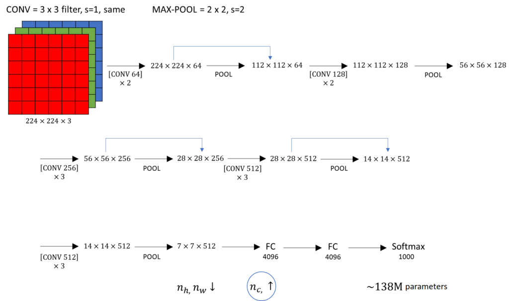
So we send these images through the pre-trained classifier. We extract a feature vector at some of the last fully connected layers in the network and this gives us a high-level semantic representation of what is in the image. It turns out that if we actually do gradient descent on this feature vector rather than on the pixels of the image or approach does work.
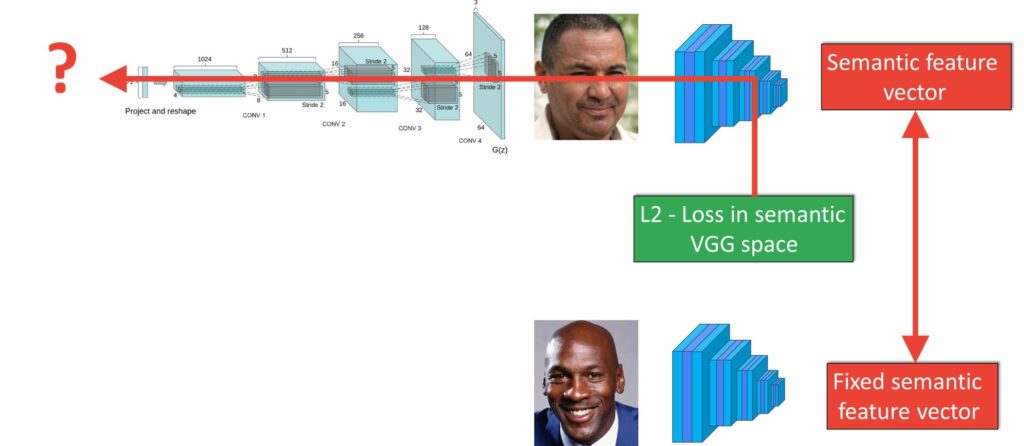
To give you an idea of what that looks like here’s a small video of an optimization process on three query images below. The top images start from the average face in the Style GAN space and then start going towards the query images at the bottom.
Now there is one final problem with this approach and that is that this is actually really really slow. It takes a very long time for the optimizer to actually find a good latent code. So, is there a way to make a really good guess of the starting point where we start our search in the latent space? With that idea why don’t we make a data set? First, we’ll sample a whole bunch of random vectors, we’ll send them through the generator, and will generate faces. Once we have that data set we can train a ResNet to go from the images to their respective latent code. So, there is already a pre-trained ResNet like this.
Here’s what our pipeline currently looks like. We take a query image. We send it through the residual network, and this network gives us an image estimate of the latent space vector in the Style GAN network. We then take that latent vector, send it through the generator which gives us an image. In this image, we apply a pre-trained VGG network in order to extract features from it. And we do the same thing for our query image of Barack Obama. Then in that feature space, we start doing gradient descent. We minimize that \(L2 \) distance in this feature space. Then we send those gradients through the generator model all the way back into our latent code. Importantly during this optimization process, the generator weights themselves are completely fixed. The only thing we’re updating is the latent code at the input of our generator.
Now in this optimization process, there are a lot of different things that you can tweak. For example which specific layer of the VGGnetwork are you using as that semantic feature vector. Or are we applying a mask to the face such that only pixels within the face region are actually used to compute that \(L2 \) difference? We can even add a penalty on the latent code that we’re optimizing such that it doesn’t move too far away from the concept of a face according to the Style GAN network. Because as it turns out you can use this process to find any image you want inside the Style GAN network. Even a Style GAN trained on faces by doing this approach you could basically find a car inside the latent space of Style GAN. But the problem is that the vector which gives you a car is going to be very far away from that Gaussian distribution that we actually started from.
So if we later want to start manipulating this face it’s gonna be a really good idea to make sure that whatever latent vector we’re gonna find is going to be similar to the concept of a face inside this Style GAN network.
We start with a query image. We send it through the ResNet and we get an initial estimate. Then we do this latent space optimization until we finally get our optimized image which is as close as possible to the query image that we started from.
Here are three additional videos of that process in action on Albert Einstein, Emilia Clark, and Barack Obama.
Now that we have the latent code which gives us our query image or at least something very close to it, what do we do now? Well now, it’s time to play. But in order to play with the latent space, we need another data set. Because what we want to do here basically is we want to start messing with specific attributes of those faces. Things like age, gender, smiling, glasses, and all of those attributes that we kind of know are important for how a face actually looks. So again we’re gonna randomly sample a whole bunch of these latent vectors. We’re gonna send them through the generator, get our faces, and then we’re gonna apply a pre-trained classifier that was trained to recognize a whole bunch of these attributes. If you wanted to you could hand label these images with any kind of attribute that you care about.
So now that we have all of those labels for the faces what do we do with them? Well basically if you look at the Style GAN latent space this is a 512-dimensional space. So it’s very complicated. And what we really care about is how a certain direction in that latent space changes the face that comes out of the generative model. So with the data set that we just created, we can basically put all of those faces at their respective locations, and we can start looking at all of the attributes that we’ve collected. All of those attributes are quite well separable by a relatively simple linear hyperplane in that latent space. Once we found that hyperplane if we take the normal with respect to that hyperplane, well this direction in the latent space basically tells us how we can make a face look more female. Because the only thing we have to do now is to take our query image, find its latent space vector, and then from that point in latent space we start walking in the direction of what makes a face more female. In the code, you will see that in the repo we’re using a whole bunch of these latent space directions that have already been predefined for you.
Summary
So, that is all. In this post, you have learned the architecture of the GANs and the theory behind the most important functions. We have also talked about amazing state-of-the-art techniques, and we learned to manipulate and play with a latent space of the most powerful generative models that we have available today.
References:
[1] Goodfellow, Ian, et al. “Generative adversarial nets.” Advances in neural information processing systems 27 (2014).
[2] Arxiv Insights YouTube https://www.youtube.com/watchv=dCKbRCUyop8&t=568s&ab_channel=ArxivInsights