#001 RNN – Recurrent Neural Networks

Highlights: Recurrent Neural Networks (RNN) are sequence models that are a modern, more advanced alternative to traditional Neural Networks. Right from Speech Recognition to Natural Language Processing to Music Generation, RNNs have continued to play a transformative role in handling sequential datasets.
In this blog post, we will learn the fundamental theory of Recurrent Neural Networks, the motivation for its use, and basic notation. So, let us start, shall we?
Tutorial Overview:
- Fundamental Concept of RNN
- Real Life Examples of RNN
- Speech Recognition
- Music Generation
- Sentiment Classification
- DNA Sequence Analysis
- Machine Translation
- Video Activity Recognition
- Name Entity Recognition
- Different Scenarios for Use of RNN
- Different Scenarios for Use of RNN
- Notation Used For Sequence Models
- Representation of Input-Output Sequence
- Representation of Words In Natural Language Processing
1. Fundamental Concept of RNN
Let us begin to understand the basis behind the introduction of Recurrent Neural Networks and how they are being implemented in some practical use cases.
Recurrent NN Vs Traditional NN
In the case of traditional neural networks, each pair of input \(x \) and output \(y \) is independent of the other input-output pairs. However, in the case of RNN, there is something called a ‘Hidden State’ that remembers the output of the previous step and treats it as the input for the next step. Simply put, Recurrent Neural Networks are a kind of sequence model that also has a memory.
2. Real-Life Examples of RNN
As you learned that RNN has a memory of their own, their major application is in sequential data. Let us look at a few examples of where RNN and such sequence models are being used.
a) Speech Recognition
When we are tasked with the transcription of audio to text, we realize how the whole audio is nothing but a collection of sequential data. Both, the input audio \(x \) that plays over time, and the output text \(y \) are a sequence of words that need to be mapped. Sequence models such as Recurrent Neural Networks along with its other variations have proven to be extremely useful for Speech Recognition.

b) Music Generation
Unlike the example of speech recognition, the problem of Music Generation has only the output as ‘sequence data’. To generate the music we like, all we need as an input \(x \) is an integer value that corresponds to a specific genre of music or the starting notes of the kind of music we want, or the input can even be an empty set. However, the output \(y \) generated will always be a sequence.

c) Sentiment Classification
Suppose you are given a review for a recently released movie or a play. The task at hand is to understand, predict, and convert this text review into a star rating for the movie or play. Such Sentiment Classification involves a sequential input \(x \), which can be as simple as a short phrase like “Entertaining, but only a one-time watch”. How would you train a model to predict the output \(y \) i.e., the number of stars this review would translate into? Understanding the likes and dislikes of the review text is handled by sequence models such as Recurrent Neural Networks.

d) DNA Sequence Analysis
Consider this. Say, your DNA is represented using four alphabets – A, C, G, and T. Given a DNA sequence input \(x \), Recurrent Neural Networks can predict which part of this sequence corresponds to a protein, output \(y \).

e) Machine Translation
In an automated language translation using a machine, sequence models such as Recurrent Neural Networks can be highly useful and efficient. Let us say you are given an input \(x \) in Latin that reads, “El que no arriesga, no gana.” Using Recurrent Neural Networks for Machine Translation, you will now need to convert this Latin input into an English output \(y \) such as this, “If you don’t take risks, you cannot win.”

f) Video Activity Recognition
Moving on to another example where the input \(x \) is in sequence form but the output \(y \) is a prediction or identification of the input sequence. Video Activity Recognition makes use of sequence models such as Recurrent Neural Networks to comprehend each video frame in the input sequence and gives a result that identifies the activity associated with that sequence.

g) Name Entity Recognition
To solve the problem of finding or identifying names of people in the given input sentence \(x \) (sequence of words), RNNs are frequently used as preferred sequence models. The task at hand for these Recurrent Neural Networks is to predict these names of places or people as output \(y \), accurately and precisely.

Let us now summarise all the examples above to create all possible circumstances under which the use of RNN can be made.
3. Different Scenarios for Use of RNN
The above examples show how diverse the applications of Recurrent Neural Networks are. Notice how in all the cases above, we are given labeled data. This means each of them falls under the domain of Supervised Learning. Looking at the use cases above, the following scenarios arise for sequence models such as RNN to be applied:
- Input \(x \) and Output \(y \) are both sequences
- Input \(x \) and Output \(y \) have same lengths
- Input \(x \) and Output \(y \) have different lengths
- Only Input \(x \) is a sequence
- Only Output \(y \) is a sequence
Now that we have learned the basic principles of Recurrent Neural Networks (RNN), let us understand how to properly describe our sequential datasets.
4. Notation Used For Sequence Models
Representation of Input-Output Sequence
The next step, after learning the theory of Recurrent Neural Networks, is to define a notation that will be used to build these sequence models.
Let us start with an example.

Luke Skywalker and Darth Vader are characters from the Star Wars. And they are here to help us solve a sample Name Entity Recognition problem using sequence models such as Recurrent Neural Networks (RNN). Such characteristic models are used by search engines to index, say, all the latest news regarding each person mentioned in the news articles, in an appropriate and structured manner. These Name Entity Recognition systems can be used to output anything from people’s names to company names to time locations, country names, currency names, and so on.
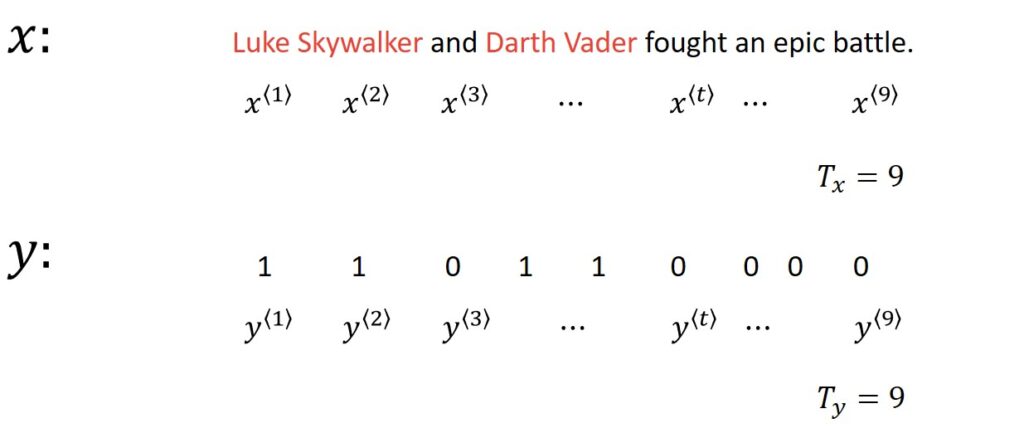
Coming back to Star Wars. “Luke Skywalker and Darth Vader had an epic battle” – consider this as an input sentence \(x \) based on which you would like to build a sequence model. This model should, then, automatically give you an output \(y \) with all the people’s names mentioned in the sentence. Each output \(y \) will identify which input word forms a part of a person’s name.
However, this is not an ideal input-output representation since there are many more sophisticated representations that not just inform you whether an input word is part of a name but also tell you where in a particular input sentence, a name starts and ends.
In our example, the input \(x \): “Luke Skywalker and Darth Vader had an epic battle” is a sequence of nine words. Therefore, this model will have nine sets of features indexed into each position of the sequential data such as \(x^{\left \langle 1 \right \rangle} \), \(x^{\left \langle 2 \right \rangle} \), \(x^{\left \langle 3 \right \rangle} \) and so on, up to \(x^{\left \langle 9 \right \rangle} \). We will assume \(t \) as a temporal sequence, whether it is temporal or not, to represent a position \(x^{\left \langle t \right \rangle} \) in the middle of the sequence. In similar way, we will notate each output of this model as \(y^{\left \langle 1 \right \rangle} \), \(y^{\left \langle 2 \right \rangle} \) , \(y^{\left \langle 3 \right \rangle} \) and so on up to \(y^{\left \langle 9 \right \rangle} \).
Adding to what we have already notated, we will introduce two more notations, \(T_{x} \) and \(T_{y} \). Here, \(T_{x} \) denotes the length of the input sequence, which in the case of this nine-word sentence is 9. And \(T_{y} \) denotes the length of the output sequence. In this example, \(T_{x} \) is equal to \(T_{y} \) but in cases such as in Machine Translation, \(T_{x} \) and \(T_{y} \) will and can have different values.
The thing to note in the above notation is that in order to represent a training example \(i \), we write it as \(x^{\left ( i \right )}\). Thus, to represent the \(t \) element of the sequence of training example \(i \), we will make use of the notation \(x^{\left ( i \right )\left \langle t \right \rangle} \). Now, if we want to denote the length of training example \(i \), we would write it as \(T_{x}^{\left ( i \right )} \). We could denote the output sequence for the training example \(i \) in a similar way as \(y^{\left ( i \right )\left \langle t \right \rangle} \) and the length of this output sequence as \(T_{y}^{\left ( i \right )} \).
Now that we have learned how to denote both, the input and the output sequences with a nice Star Wars example, let us continue to explore more notations, specifically, when it comes to words in Natural Language Processing.
Representation of Words in Natural Language Processing
An important thing to learn when working with cases such as Natural Language Processing is how to represent individual words of the given input sequence.
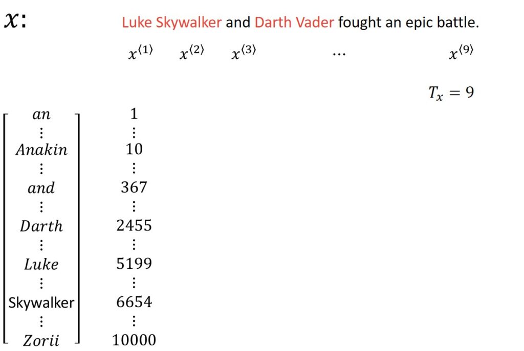
Continuing with the above input sequence, “Luke Skywalker and Darth Vader had an epic battle”, we will now see how we can represent, say, the word “Luke”. To understand the why, what, and how of the notation we learned earlier \(x^{\left \langle 1 \right \rangle} \), we need to make a comprehensive list of all words into a vocabulary or a sort of dictionary.
This is how we do it:

Look at the dictionary above and notice how it starts with the word “a” and ends with the last word of the dictionary “Zorii”. We can then denote numerical values to each of these words according to the dictionary order, starting with “a” being 1, “Anakin” being 10, and so on till the 10,000th index position for “Zorii”.
Currently, we have assumed this dictionary to be a collection of a total of 10,000 words. However, for reasonably sized commercial applications, dictionary sizes of 30,000 to 50,000 are more prevalent. You may come across applications where even a dictionary size of 100,000 words looks more suitable. In the case of large internet companies, these dictionary sizes go up to a million words plus. But don’t worry, for our illustration and understanding, we’ll stick to 10,000 words for now.
Now, the question arises, how do we choose these 10,000 words? Well, one way to build the dictionary is to find the topmost occurring words within our training sets. We can also look at the 10,000 most common English words in any of the popular online dictionaries.
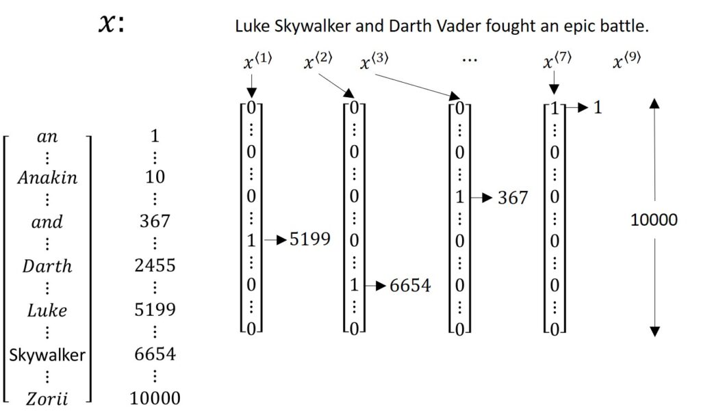
Look at the graphical representation of our one-hot dictionary mapping.

Note how \(x^{\left \langle 1 \right \rangle} \) which represents the word “Luke” is a vector with all zeros except for a single 1 at position 5119 since that is the position of the word “Luke” in the dictionary we made. Similarly, “Skywalker”, represented by \(x^{\left \langle 2 \right \rangle} \), is a vector of all zeros except for the position 6654 where it is 1. And so on. Each of these vectors will be a 10,000-dimensional vector, according to what your dictionary size is.
All represented \(x^{\left \langle t \right \rangle}\) for each value of \(t \) in the example sentence we have, will be One-Hot Vectors. This is because all values in these vectors are zero except for one value which is 1. In our example, we have nine such One-Hot Vectors that represent the nine words of the example sentence. Our main objective is to map this $ latex x $ using a sequence model and achieve our target output \(y \). There is, however, one little problem. What if we come across a word that is not listed in our dictionary? Well, in that case, we can create ‘Unknown Words’, new (fake) words in the form of tokens, that we denote using angle brackets UNK.
So, what do we have? We have a lot of labeled data at hand, now. Don’t you think it is wise to consider this as a Supervised Learning Problem? You are right. In the upcoming tutorial blogs, we will look at how cases such as Natural Language Processing can be worked on using sequence models like Recurring Neural Networks and the technique we already know so well, Supervised Learning.
How was it learning about Recurrent Neural Networks? I hope you gained deeper insights into a more modern technique of handling sequential data, as compared to traditional neural networks. Now, that you also know how to represent this data using appropriate notations, we will soon get on to building our own RNN models, solving real-life cases. Exciting, isn’t it?
Recurrent Neural Networks
- Types of Sequence Models
- More advanced than traditional Neural Networks
- Best at handling sequential data, either sequential input or output or both
- Have a memory of their own
- Wide range of real-life applications
Summary
Well, folks, that’s it for this post! Recurrent Neural Networks (RNN) are now a familiar thing for you, I’m sure. Don’t be shy and read more about how to map input and output sequences in different ways. Of course, we will take that journey together too, so, be prepared. Till then, May The Force Be With You! ?