#001 Deepfakes – Understanding Generative Learning

Highlights: The evolution of Generative Adversarial Networks (GANs) has brought about a change in how researchers solve certain Computer Vision problems such as conditional image generation, 3D object generation, video synthesis, and more.

In this tutorial blog post, we will go into detail about the fundamentals of generative learning, its categories, and the different types of GANs that are popular in the Computer Vision field of research. So let’s begin!

Tutorial Overview:

1. Generative Learning
2. Vanilla GAN (2014)
3. Conditional GAN (2014)
4. Deep Convolutional GAN (2015)
5. InfoGAN (2016)
6. Training GANs (2016)
   

1. Generative Learning

Introduction

From computer vision to natural language processing, generating data that are indistinguishable to the human eye is a major application of data generation methods using Generative Learning.

Broadly, there are two main categories of Generative Learning:

1. Variational AutoEncoders (VAE)
2. Generative Adversarial Networks (GAN)

The use of GANs makes it look like the researchers are making things complicated. The use of autoencoders could easily minimize the mean squared error such that the target image can match the predicted image. So, why aren’t autoencoders used without any hassle of GANs?

First, the autoencoder model doesn’t produce great results when it comes to image generation. Simply minimizing the error produces predictions that are blurry. This is due to the fact that the loss, which is the average quantity of all pixels, is a scalar value.

Second, the method wherein autoencoders are used doesn’t produce diverse results as effectively as GANs.

To understand how GANs work, let’s go over the basics of adversarial learning.

Adversarial Learning

A slight change in the input to a deep learning model during testing can reduce the performance of image classification. This vulnerability of deep learning models from even the smallest of noise can generate results that are indistinguishable but are incorrectly classified.

To address this problem, we inject adversarial examples into the training set to increase the robustness of the network. In such examples, noise is added by applying data augmentation techniques or by perturbing the image in the opposite direction of the gradient. This maximizes the loss instead of minimizing it.

There is another way to address the same problem. Instead of using a robust classifier, we can let the network create different examples that are visually appealing. This is the generative technique and is performed within the network using a ‘Generator’.

Let’s understand the term ‘Generator’ and its functions better using examples of different kinds of Generative Adversarial Networks (GANs).

2. Vanilla GAN

Generator

A generator is simply a neural network that requires input and we can decide what output we want. A random noise, sampled from a distribution in a small range of real numbers (also known as latent or continuous space), is given as input and a non-deterministic output is received for each input.

This is what we call ‘Stochasticity’, wherein, there is no limit to the number of samples we can generate. Using this, we can focus on generating representative examples of specific distribution such as cats, trains, and art pieces, among others.

Discriminator

A discriminator is essentially a classifier that focuses on learning class distribution and quantifies how representative the class is of the real class distribution. The output of the discriminator is a probability value such that 0 represents the fake generated images and 1 denotes the real samples from our distribution.

0.5 is the ideal output when the generator produces indistinguishable examples. This example is also true in Game theory which talks about a non-cooperative game between two players, known as the Nash Equilibrium or a minimax game. Here, we assume that each player knows the equilibrium strategies of the other player and no player has anything to gain by changing their own strategy.

In order to fool Discriminator D, fake examples that are close to the real distribution are produced by Generator G. The discriminator, then, tries to guess and decide the origin of the distribution. This means that the discriminator is getting updated dynamically based on ‘indirect’ training.

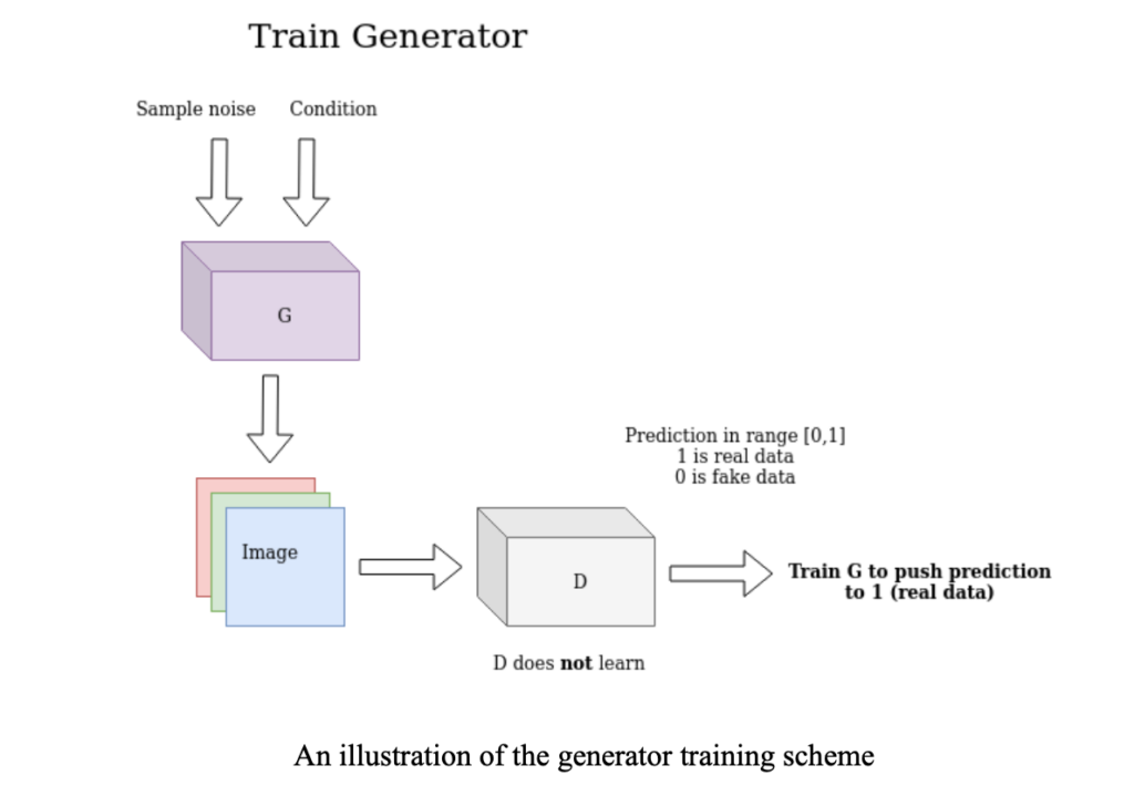
This is the core idea of a Generative Adversarial Network (GAN). In short, in a GAN, a generator is trained to fool the discriminator instead of minimizing the error, using unsupervised learning. Have a look at the generator training scheme below.

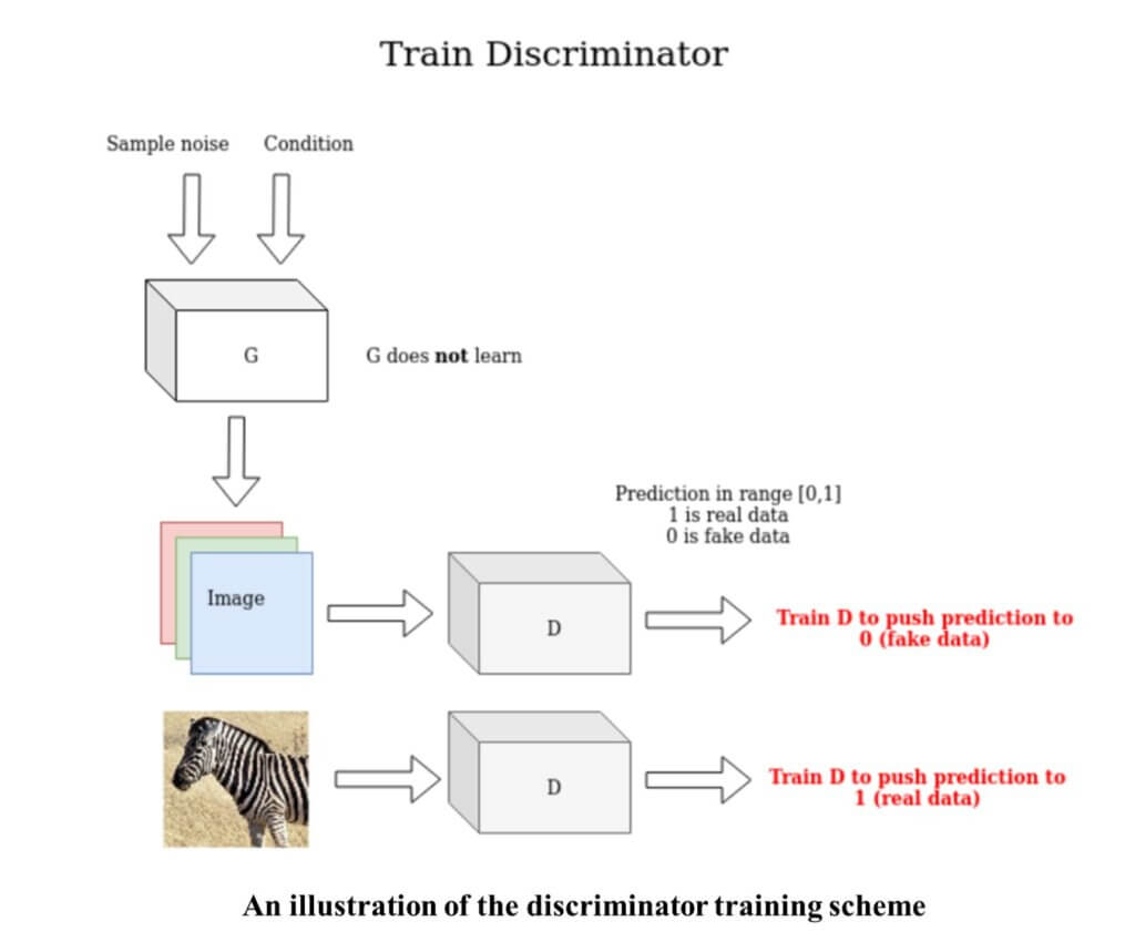
The discriminator uses the real and the generated image and tries to distinguish between the two. Have a look at the discriminator training scheme below.

In 2014, the authors of GAN proposed an architecture that consisted of 4 fully connected layers for the generator as well as the discriminator, wherein the output of the generator is a 1-dimensional vector and the output of the discriminator is a scalar value between 0 and 1.

Let us see how GANs are trained, in terms of mathematical representation.

Given \(D \), our discriminator, and \(G \), our generator, we can define V, the value function of our two-player minimax game, for \(M \) samples, as follows:

$$ \min _G \max _D V(G, D)=E_{\mathbf{x} \sim p_{\text {data }(\mathbf{x})}}[\log D(\mathbf{x})]+E_{z \sim p_{\text {fake }(z)}}[\log (1-D(G(z)))] $$

The expected value is represented using the following expression:

$$ L_D=\frac{1}{M} \sum_{i=1}^M\left[\log D\left(\mathbf{x}^i\right)+\log \left(1-D\left(G\left(\mathbf{z}^i\right)\right)\right)\right] $$

$$ L_G=E_{z \sim p_{\text {fake }(z)}}[\log D(G(z))]=\frac{1}{M} \sum_{i=1}^M\left[\log \left(D\left(G\left(\mathbf{z}^i\right)\right)\right)\right] $$

Notice that the generator which performs gradient descent has no access to the real images. And, the discriminator which performs gradient ascent has access to the real as well as the fake images. Have a look at the python code below.

import torch

def ones_target(size):
    '''
    For real data when training D, while for fake data when training G
    Tensor containing ones, with shape = size
    '''
    return torch.ones(size, 1)

def zeros_target(size):
    '''
    For data when training D
    Tensor containing zeros, with shape = size
    '''
    return torch.zeros(size, 1)


def train_discriminator(discriminator, optimizer, real_data, fake_data, loss):
    N = real_data.size(0)
    # Reset gradients
    optimizer.zero_grad()
    # Train on Real Data
    prediction_real = discriminator(real_data)
    # Calculate error and backpropagate
    target_real = ones_target(N)

    error_real = loss(prediction_real, target_real)
    error_real.backward()

    # Train on Fake Data
    prediction_fake = discriminator(fake_data)
    # Calculate error and backpropagate
    target_fake = zeros_target(N)

    error_fake = loss(prediction_fake, target_fake)
    error_fake.backward()Code language: PHP (php)

    # Update weights with gradients
    optimizer.step()
    return error_real + error_fake, prediction_real, prediction_fake


def train_generator(discriminator, optimizer, fake_data, loss):
    N = fake_data.size(0)
    # Reset the gradients
    optimizer.zero_grad()
    # Sample noise and generate fake data
    prediction = discriminator(fake_data)

    # Calculate error and backpropagate
    target = ones_target(N)
    error = loss(prediction, target)
    error.backward()
    optimizer.step()
    return errorCode language: PHP (php)

The above code produces the following results, in the form of generated images where each change corresponds to a different epoch.

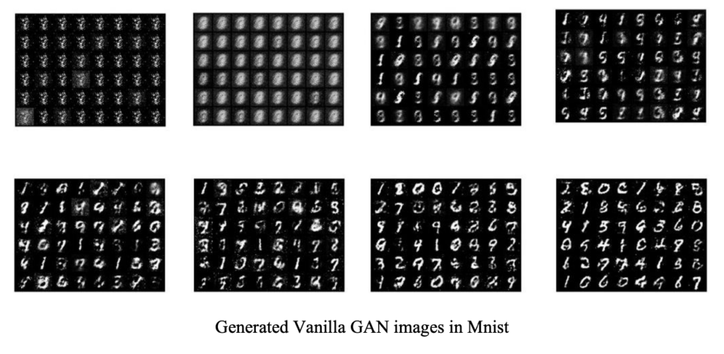
The Mode-Collapse Problem

Often, the generator fails to represent the pixel-space of all the possible outputs and instead, selects only a few influential modes that correspond to noise images. This results in a highly unstable generator due to exploding gradients. Seeing the generator collapse, the discriminator pushes a single point that is being emitted by the generator around the space forever.

Mode collapse can also happen when the discriminator gets stuck in a local minimum and the generator finds it extremely easy to fool the discriminator.

In terms of the game theory, mode collapse is the state in which one of the players gains an almost irreversible advantage, making it difficult for that player to lose the game.

Now, let us move ahead and learn about another type of GAN known as the Conditional Generative Adversarial Network.

3. Conditional GAN (2014)

Suppose a certain event has already occurred. Now, if we were to calculate the probability of a second event occurring after the first event has occurred, we’ll call it Conditional Probability.

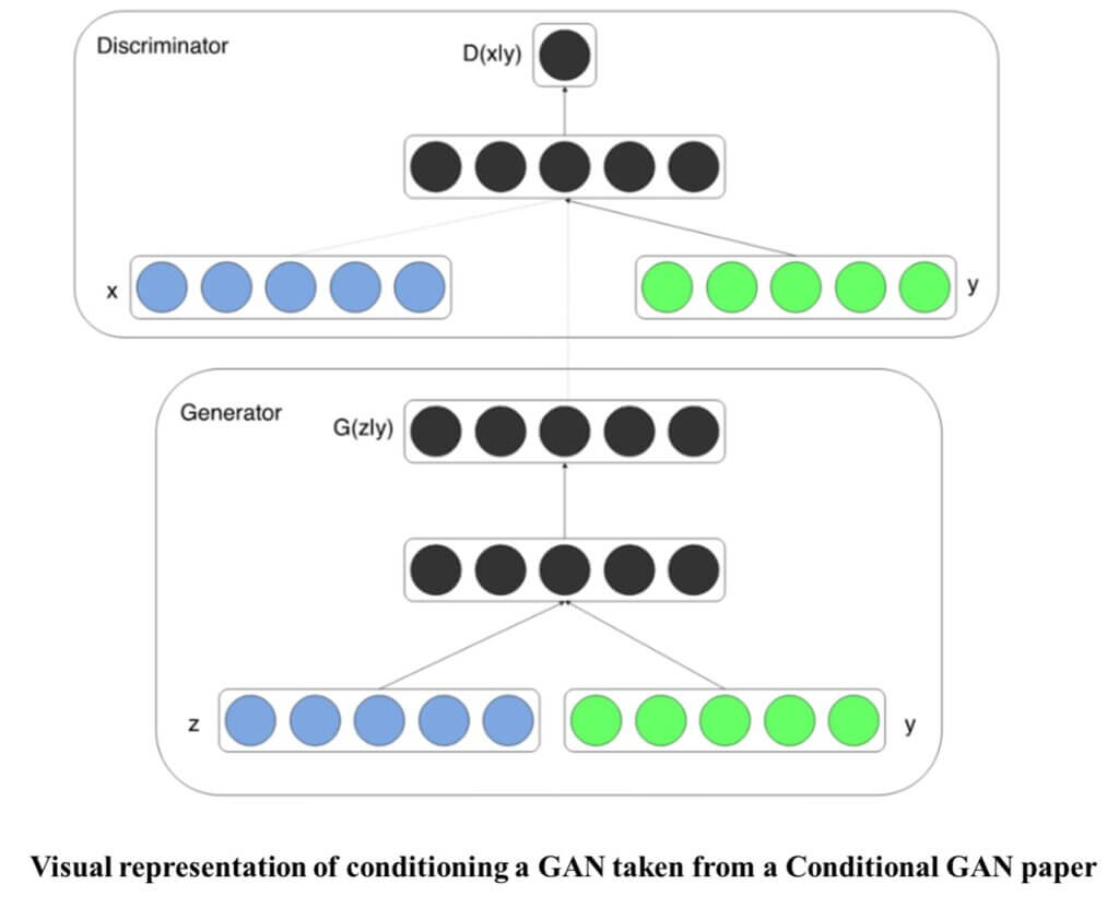
Conditional GANs make use of conditional information based on extra data or ‘auxiliary’ information such as image tags, and labels, among others, to guide the data generation process. Concatenation is used to feed this additional input into the generator as well as the discriminator.

Semantic segmentation is a form of conditioning used in medical image generation that utilizes demographic information such as age, height, and more.

Have a look at the visual representation of Conditional GAN below (source: https://arxiv.org/pdf/1411.1784.pdf).

As the GANs evolved, newer types of networks came into the picture. Let us learn about a first-of-its-kind GAn that was proposed in 2015 and became popular since then.

4. Deep Convolutional GAN (2015)

DCGAN was the first Convolutional Generative Adversarial Network that was introduced in 2015. In this topologically constrained GAN, a few modifications were made in previous versions of GANs to achieve a reduced number of parameters per layer and to make the training faster and more stable.

Following are some guiding principles of DCGANs:

• In the discriminator, all Pooling layers are replaced with convolutions. While it increases the model’s expressiveness, it also increases the number of trainable parameters.
• In the generator, transpose convolutions are used to increase spatial dimensions and reduce the number of feature maps.
• In the generator as well as the discriminator, batch normalization is used to stabilize training and enable a higher learning rate.
• In deeper architectures, fully-connected hidden layers are removed in order to reduce the number of training parameters and training time.
• In the generator, ReLU activation is used for all layers except for the output.
• In the discriminator, LeakyReLU activation is used for all layers to enable the model to learn more complex representations.
• In the discriminator, fewer feature maps are used than the compared method (K-means).

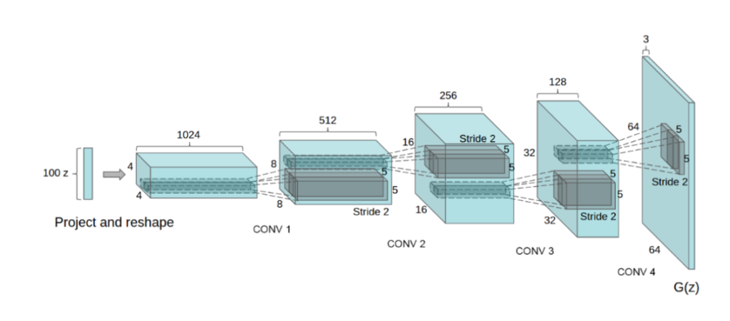
Here’s what a typical DCGAN architecture looks like.

When implemented using code, a sample DCGAN model in the MNIST dataset gives the following results. Have a look.

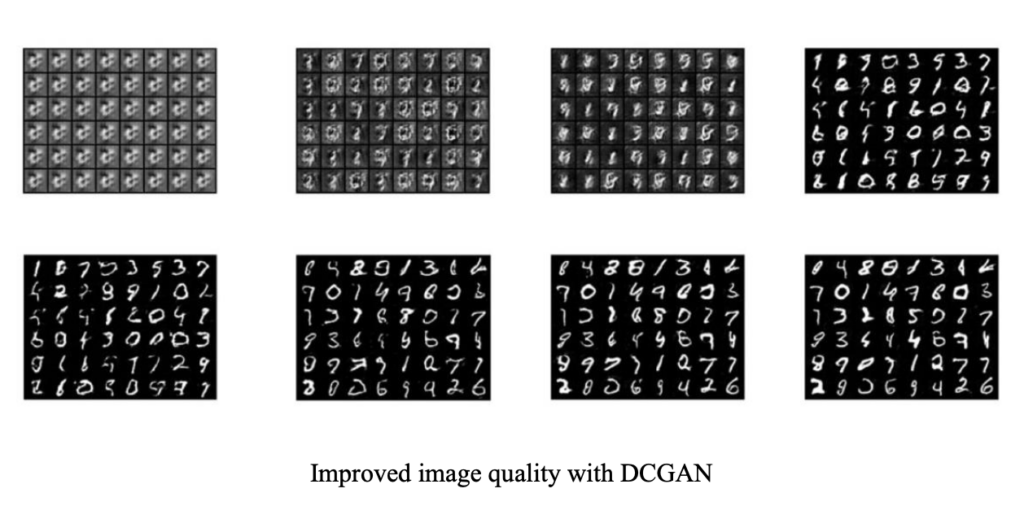
Notice how the output is crisper and less noisy. This is due to the convolutional layers.

Mode collapse also happens in DCGANs. In the image below, the researchers tried to train a DCGAN in CIFAR-10 using only one class. Have a look at the result.

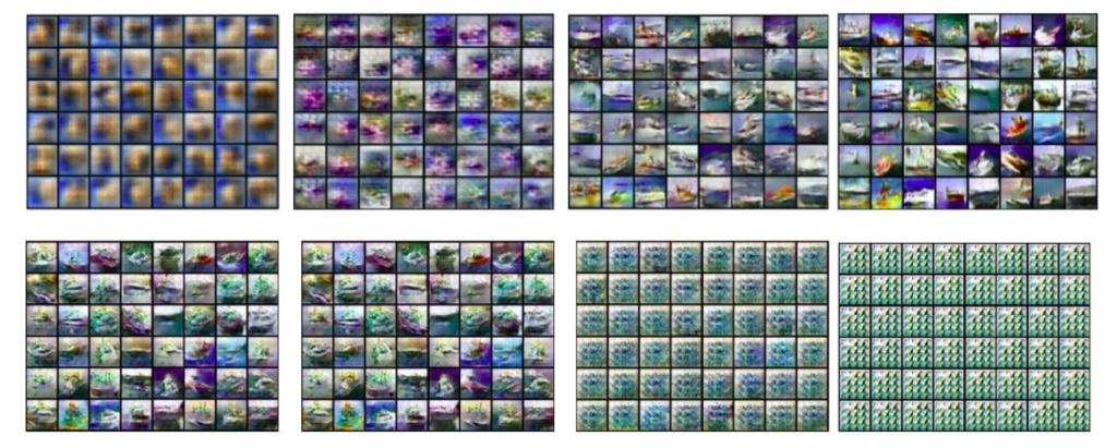
In the result above, observe how the generator starts to collapse towards the end when started with a noise and ends up outputting a repetitive square pattern.

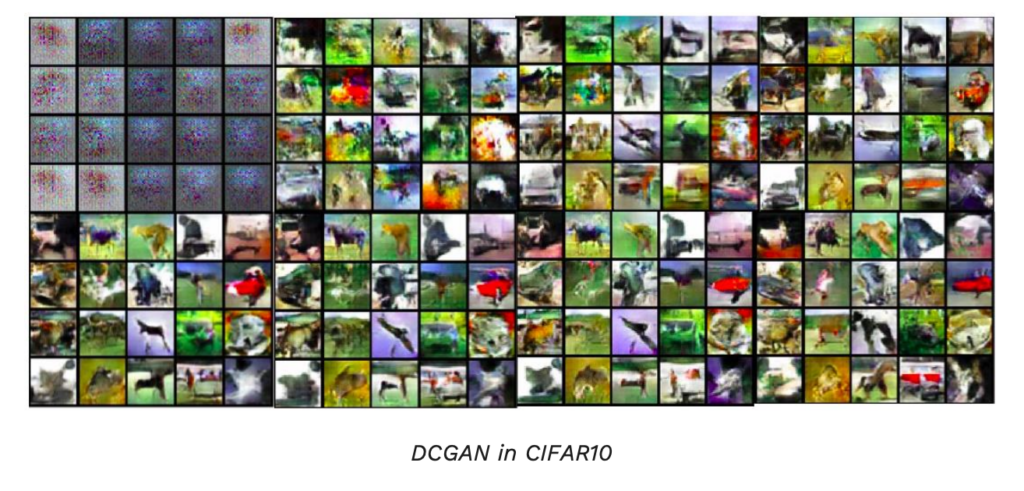
However, once we train DCGAN on the entire CIFAR-10 dataset using all the classes, we get a result that looks like this.

Let’s move on to the next kind of GAN.

5. InfoGAN (2016)

InfoGAN refers to Information Maximization of learning disentangled representation of images in Generative Adversarial Networks. Unlike Conditional GANs, where we need to provide labels to our datasets on our own, InfoGAN works on the model of unsupervised learning, deriving labels automatically from the datasets.

InfoGANs work using two basic principles.

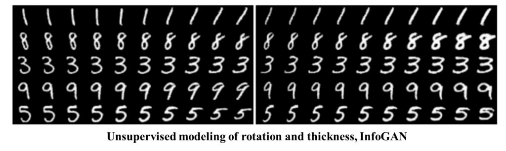
1. Disentangled Representations: This is an unsupervised learning technique that breaks down each feature into narrowly defined variables and encodes them as separate dimensions.
   
2. Mutual Information: The quantitative measure of the mutual dependency between two random variables is known as Mutual Information. This reduces the uncertainty in the generated output when the conditional random variable is observed.

Have a look at the unsupervised modeling of rotation and thickness for a sample InfoGAN implementation.

There are many ways of training GANs with a variety of new architectural techniques and training procedures. Let’s study some of them.

6. Training GANs (2016)

In terms of game theory, training of GANs involves finding a two-player Nash equilibrium. However, many times, the gradient descent fails to converge due to the non-convex nature of the cost function and parameters being continuous. This means that the parameter space is extremely high-dimensional.

This high-dimensional path is known as the ‘Manifold’, which is essentially the set of generated images that satisfy our objective.

Suppose we want to find a really small subset of the world that represents human faces. In our objective of learning human faces, we move on a path along the vectors’ solutions, each vector representing each face.

There are many tricks to train Generative Adversarial Networks (GANs). Here are a few:

1. Feature Matching: Here, the generator is trained to match the expected value of the features on an intermediate layer of the discriminator. This method is effective when regular GANs become unstable.
   
2. Minibatch Discrimination: This method is used to generate visually appealing samples extremely quickly since the discriminator processes each example independently and there is no correlation between its gradients. The method also allows the discriminator to look at multiple data examples and quantifies a measure of pairwise similarity for each data pair.
   
3. Historical Weight Averaging: Low-dimensional problems where gradient descent may fail, this method can work effectively.
   
4. Inception Score: This quantitative method to evaluate a model instead of inspecting visual quality one by one can be used to infer the label using conditional probability and measure the KL divergence of the classifier compared to unconditional probability.
   
5. Semi-Supervised Learning: Here, samples from the GAN generator are added to the dataset with a ‘generated’ class label, given that the pre-trained classifier recognizes the label with low entropy.
   
   

So this was the entire post on different concepts around generative learning, adversarial learning, and GAN training schemes. We also discussed mode collapse, conditional generation, and disentangled representations based on mutual information.

You can continue to learn using this amazing repository: https://github.com/kwotsin/mimicry

You can also check out this very informative course on Udemy: https://www.udemy.com/course/deep-learning-gans-and-variational-autoencoders/?awc=6554_1629724057_d152302f6e61e03d97b17fd56d0f29b4&utm_source=Growth-Affiliate&utm_medium=Affiliate-Window&utm_campaign=Campaign-Name&utm_term=683487&utm_content=Placement

Understanding Generative Learning

• Generative learning helps in producing nearly indistinguishable generative data
• There are two types of generative learning – Variational Autoencoders (VAE) and Generative Adversarial Networks (GAN)
• Ordinary AutoEncoders produce poor results when it comes to image generation
• Adversarial examples are included in deep neural networks using a Generator
• A generator’s main job is to fool the discriminator
• GANs are based on unsupervised learning
• Vanilla GANs, Conditional GANs, Deep Convolutional GANs, and InfoGANs are some of the different types of GANs that have been used since 2014
  

Summary

That’s it, folks! Do let us know how you like this post on the fundamentals of Generative Learning. Mention in the comments what kind of dataset would you like to apply these ideas to. This is just the beginning of this GAN series and we’ll cover a lot more interesting topics in the upcoming posts. Stay tuned. Until then, have some ‘unsupervised’ fun! 🙂