#012 TF Transfer Learning in TensorFlow 2.0
Highlights: In this post we are going to show how to build a computer vision model without building it from scratch. The idea behind transfer learning is that a neural network that has been trained on a large dataset can apply its knowledge to a dataset that it has never seen before. That is, why it’s called a transfer learning; we transfer the learning of an existing model to a new dataset.
Tutorial Overview:
1. Introduction
Previously we have explored how to improve the models performance using a data augmentation. The question now is, “what if we don’t have enough data to train our network from scratch?”.
A solution to this is using the transfer learning method. A more theoretical post has been posted on our blog. Check it out to refresh some ideas if needed. We can use transfer learning to transfer knowledge from some pre-trained opensource network to our own CV problem.
The computer vision research community has posted lots of datasets on the internet like Imagenet or MS Coco or Pascal datasets. Many computer vision researchers have trained their algorithms on these datasets. Sometimes this training takes several weeks and might take many GPUs. The fact that someone else has done this task and gone through the painful high-performance research process means that we can often download open source weights.
There are a lot of networks that have been trained. For example, the Imagenet dataset, which consists of 1000 different classes and over 14 million images. Hence, the network might have a softmax unit that outputs one of a thousand possible classes. What we can do is to get rid of the softmax layer and create our own output unit to represent, for instance, cat or dog.
Since we are using downloaded weights, we will just train the parameters associated with our output layer, which in our case will be a sigmoid output layer.
2. Transfer learning with a built-in TensorFlow model
Let us first prepare the dataset for the training. We are going to download dataset with wget.download command. After that, we need to unzip it and merge paths for the training and test parts.
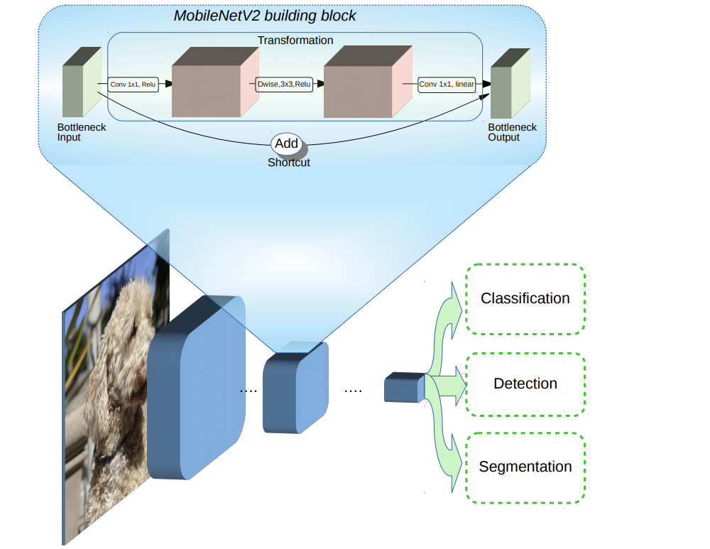
Now let’s import all required libraries and build our model. We will use a pretrained network called MobileNetV2 which is trained on ImageNet dataset. Here, we want to use all layers except the classification layers on the top, so we won’t include them in our network.

This and other pretrained models are already available in TensorFlow.
If the final layer outputs different number of classes then we need to have our own output unit that outputs the following classes: a cat or a dog. There are a couple ways to do this:
- Take the last few layers’ weights and just use them as an initialization and do the gradient descent. This way we will just retrain part of the network.
- Remove these last few layer’s weights, use our own new hidden units and our own final sigmoid (or softmax) output. In this way we can change the number of outputs.
Hence, either of these methods could be worth trying.
Let us now freeze pretrained layers and add a new layer, called GlobalAveragePooling2D and after this a Dense layer with a sigmoid activation function.

It is time for the training step. We will use an image data generator to iterate through images. Now it is not necessary to train a network for a large number of epochs because we already have a part of network pre-trained.
Let’s see the results.
3. Transfer learning with TensorFlow Hub
Another method for accessing pretrained models is TensorFlow Hub. TensorFlow Hub is a library for the publication, discovery, and consumption of reusable parts of machine learning models. You can find more pretrained models here.
We will freeze layers and add a new one for classification. The input to the fully connected network is called the bottleneck features. They represent the activation map from the last convolutional layer in the network.

Let’s train the model for a given number of epochs.
Here we can also use TensorBoard, but let’s keep it simple this time.
Finally, let’s visualize some predictions. In this dataset, cats are labeled with 0 and dogs with 1. We will display correct predictions with a blue color and false with a red color.

Summary
As we can see above, using transfer learning can help us to achieve really good results in a short period of time. Using data augmentation, the results can be further enhanced.
In the next post we will show how to create a network and transform it for use on mobile devices.