OpenCV #013 Harris Corner Detector – Experiment
Highlights: In this post we will continue working on Harris Corner Detector. In the previous post we presented the basic idea behind this algorithm, and here we will wrap this up and show how this method works in OpenCV.

Tutorial Overview:
- Interpreting the Second Moment Matrix
- Interpreting the Eigenvalues
- Harris Corner Response Function
- Harris Detector Algorithm
- Code
1. Interpreting the Second Moment Matrix
Let’s first consider the case, where the gradient at every point in the window, is either horizontal or vertical.
So, at each point, it could be horizontal or it could be vertical, but it’s not going to be slanted. So some places it’ll be horizontal, some places it’ll be vertical, but both \(I_{x} \) and \(I_{y} \) are never non-zero at the same time. Well, that would mean that \(I_{x}I_{y} \) would always be \(0 \). So, that would look like this:
$$ M= \sum_{x,y}^{ }w\left ( x,y \right )\begin{bmatrix}I_{x}^{2} & I_{x}I_{y} \\I_{x}I_{y} & I_{y}^{2}\end{bmatrix} = \begin{bmatrix}\lambda _{1} & 0\\0 & \lambda _{2}\end{bmatrix} $$
Where \( \lambda _{1} \), \(\lambda _{2}\) are the eigenvalues of \(M \). These are the diagonal terms. The off diagonals would be \(0\). Now, that’s a nice full right matrix, except if one of those were \(0\), it would not be a full rank equation. So for example, if the \(I_{y}^{2}\) were all \(0\) and that there was no gradient in the \(y\) direction, only in the horizontal direction, that would mean that our matrix would only have one of these values, and probably, that’s not really a good corner. Because if we only have gradient in one way and not in other way, then we can slide up and down as much as we want.
So, something about these numbers tells us how good a corner, the location in the image is. In fact, if either of those lambdas were close to \(0\), this is not a corner. So we want to look for locations where both of those are large.
2. Interpreting the Eigenvalues
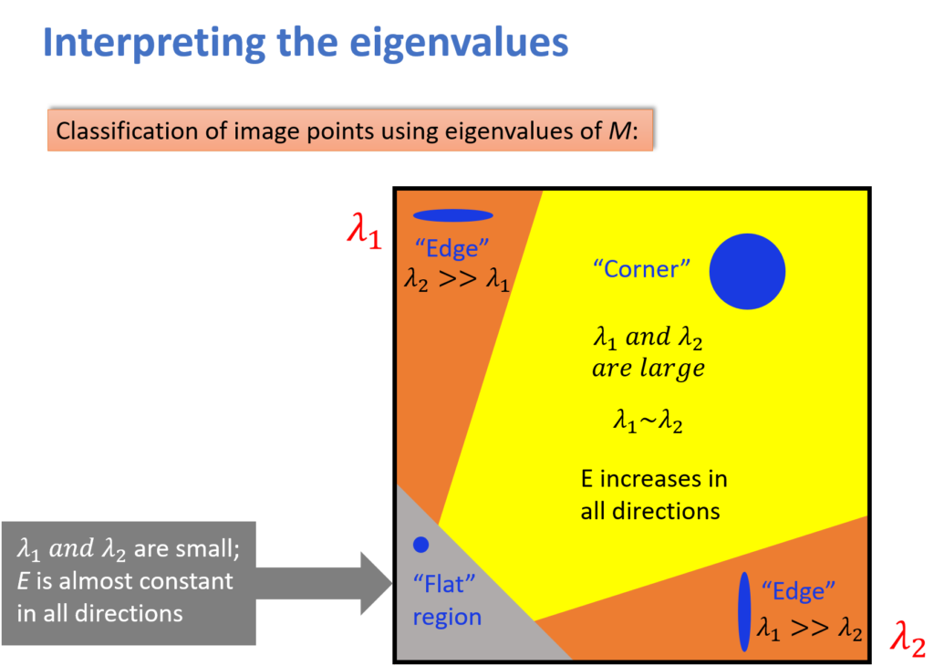
Here is how we are going to do it. The idea is that we are going to classify our image points based upon computing those, that Harris matrix, and looking at some measure that’s a function of its eigenvalues.

And the idea is that in a flat area, both of those eigenvalues will be very small. In fact, if it was perfectly flat, everything would be zero because the gradients were zero everywhere. And that would mean no matter how we moved, nothing changes, so it’s a terrible corner.
Likewise, if we have just one of the eigenvalues large, that means there’s some direction that changes quickly so if we move in that direction, we know things have changed. But if it’s zero in the other direction we can move as much as we want. That’s what happened along an edge, so when one eigenvalue is much, much bigger than the other then we are along an edge up here.
And when is it a corner? Well, when both of the eigenvalues are large. So, we want them to be approximately the same magnitude. Just that they’re both big enough, and that the ratio between them should not be terrible. If they are both large, but the ratio between them is pretty big, then probably our code was wrong and we have to worry because it means one gradient is much more dominant than the other, and maybe the noise is affecting the finding of the corner. Is that means all we have to do is find the eigenvector, and the eigenvalues? Guess what? We don’t even have to do that. This is what was so good about the Harris thing.
3. Harris Corner Response Function
We have to remember something, that the determinant of a matrix, that is actually the product of the eigenvalues. So \(\lambda _{1} \lambda _{2}\), multiply them together, that’s the determinant.
$$ R=det\left ( M \right )-\alpha trace\displaystyle \left ( M \right )^{2}= \lambda _{1}\lambda _{2}-\alpha \left ( \lambda _{1}+\lambda _{2} \right )^{2} $$
The other thing is that the trace of the matrix, the sum of the diagonals, is the sum of the eigenvalues. Trace is easy, sum them up. And the Harris operator was just to compute some function \(R\), you take the \(M \) matrix, we take its determinate, minus some constant of the square of the trace. And empirically, the constant was small number, \(0.04 \), \(0.06 \).
4. Harris Detector Algorithm
And finally, we have this algorithm:
- Compute Gaussian derivatives at each pixel
- Compute second moment matrix M in a Gaussian window around each pixel
- Compute corner response function R
- Threshold R
- Find local maxima of response function (non-maximum suppression)
5. Code
OpenCV has the function cornerHarris() for the purpose of detecting corners. It takes the following parameters:
- img – Input image, it should be grayscale and float32 type.
- blockSize – It is the size of neighbourhood considered for corner detection
- ksize – Aperture parameter of Sobel derivative used.
- k – Harris detector free parameter in the equation.
The only difference will be that C++ has a second parameter, which is the output.
Python
C++
#include <opencv2/opencv.hpp>
#include <iostream>

using namespace cv;
using namespace std;

int main()
{
    Mat image, gray;
    Mat output, output_norm, output_norm_scaled;

    // Loading the actual image
    image = imread("03.jpg", IMREAD_COLOR);

    // Edge cases
    if(image.empty()){
    	cout << "Error loading image" << endl;
    	return -1;
    }
    cv::imshow("Original image", image);
    cv::waitKey();

    // Converting the color image into grayscale
    cvtColor(image, gray, cv::COLOR_BGR2GRAY);

    // Detecting corners
    output = Mat::zeros(image.size(), CV_32FC1);
    cornerHarris(gray, output, 2, 3, 0.04);

    // Normalizing
    normalize(output, output_norm, 0, 255, NORM_MINMAX, CV_32FC1, Mat());
    convertScaleAbs(output_norm, output_norm_scaled);

    // Drawing a circle around corners
    for(int j = 0; j < output_norm.rows ; j++){
        for(int i = 0; i < output_norm.cols; i++){
            if((int) output_norm.at<float>(j,i) > 100){
               circle(image, Point(i,j), 2,  Scalar(0,0,255), 2, 8, 0 );
            }
        }
    }

    // Displaying the result
    cv::imshow("Output", image);
    cv::waitKey();
    //cv::imwrite("Detected_circles.jpg", image);
    return 0;
}
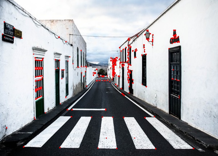
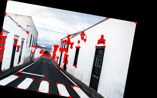
Results:

Also, this can be useful when we want to detect the image corners, which is shown in the following picture.

Summary
All things considered, we have learned a detailed procedure of how Harris Corner Detector works. As shown above, there is a lot of math, although a complicated part is skipped, thankfully OpenCV provides us a function for this.
In the next post, we will learn more about Histogram Equalization.