OpenCV #008 Canny Edge Detector
Digital Image Processing using OpenCV (Python & C++)
Highlights: In this post, we will learn about the Canny Edge Detector. In the last few posts, we explained why edges are important for better understanding of the image, and how we can use Laplacian and Sobel filter to detect them. At the places where this method does not give good results, we can use the Canny Edge Detector and dramatically improve the obtained results.
Tutorial Overview:
- Derivative of Gaussian Filter 2D
- Effect of Sigma on Derivatives
- Canny Edge Operator
- Code for Canny Edge Detector
Intro
In practice, when we try to detect edges using derivatives, high-frequency noise will produce undesirable results. Hence, it is a good strategy to first low pass an image, and only then to apply the gradient. We can do this in two ways:
- low pass an image (let’s say a low-pass Gaussian filter) and calculate a derivative
- smooth a derivative operator (apply a Gaussian filter), and then apply it to an image.
In our post we will proceed with the second method.
1. Derivative of Gaussian Filter 2D
In 2D we can’t just talk about derivatives, but we also have to talk at the direction of the derivative. In gradients, we have derivatives in the \(x \) direction and derivatives in the \(y \) direction.
We can express this in the following way:
$$ \left ( I*g \right )*h_{x}= I*\left ( g*h_{x} \right ) $$
Let’s suppose we want to take the derivative in the \(x \) direction. And what this \(h_{x} \) is meant to imply is that that is a filter that just takes derivative in the \(x \) direction. And \(g\) is going to be Gaussian. We can apply an operator that is the Gaussian with its derivative. And that gives us this function like this in the next picture.
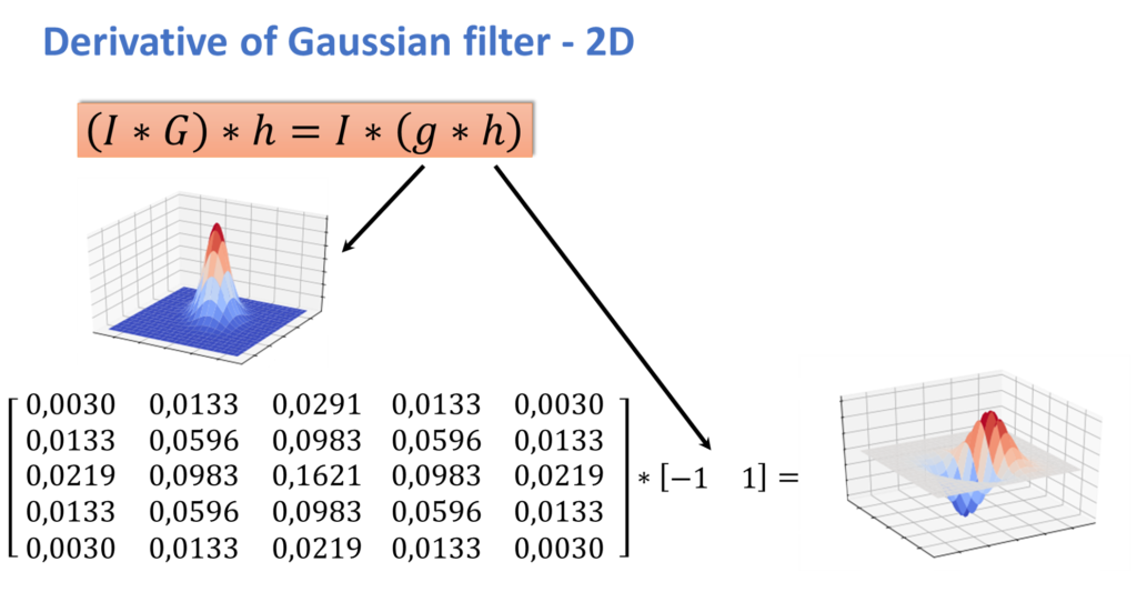
And that is the first derivative of the Gaussian, which when we apply to an image gives us the derivative of the Gaussian smooth image for that associative property from before.
2. Effect of Sigma on Derivatives
When we do this, we end up with this gradient function which is shown in the next picture. And of course, we can do this both in the \(x \) direction and the \(y \) direction.
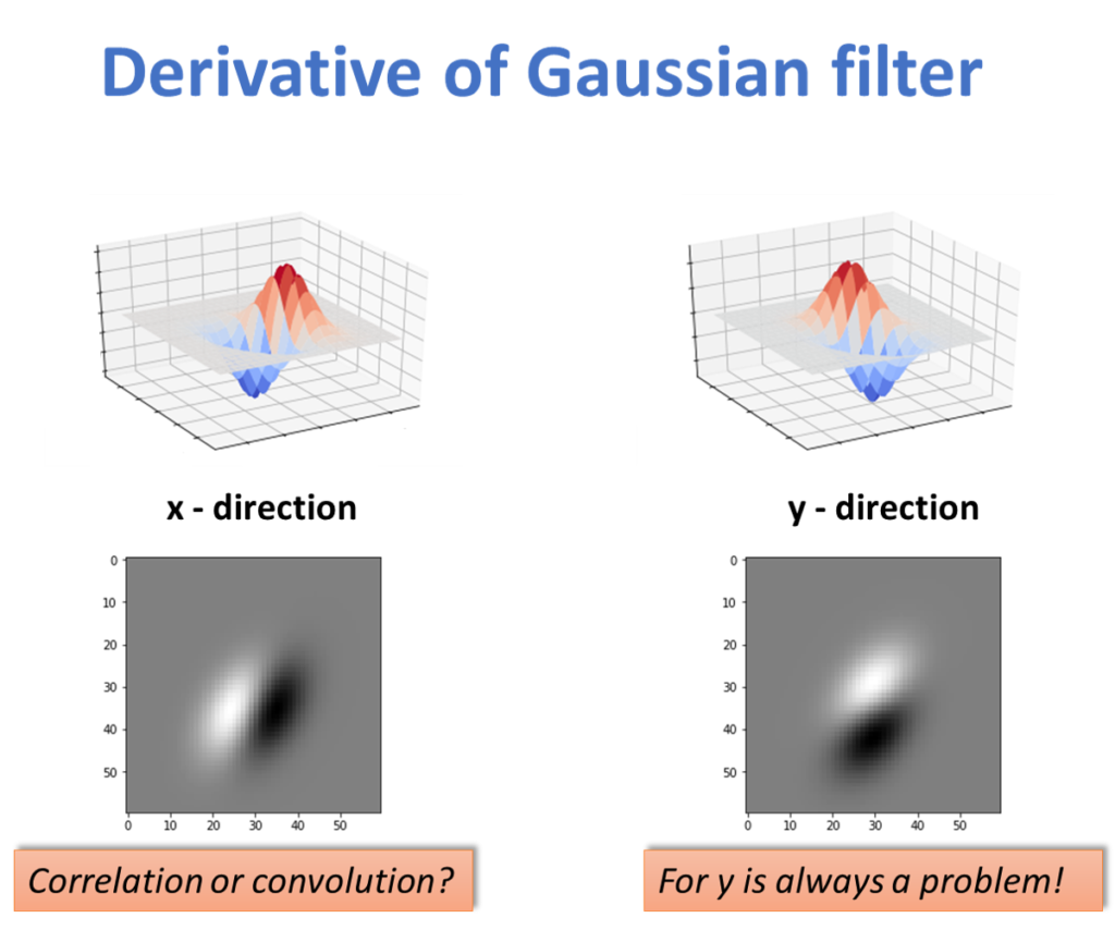
And now there is this problem of correlation versus convolution. In the \(x \) direction if \(x \) goes from left to right, this is a correlation filter. On the other hand, in the \(y \) direction, which way is positive is always a problem because \(y \) can go up or down. The main issue, of course, is that it goes vertically.
So that’s how we would use a Gaussian in order to get some smooth derivatives. But there is this question of how large Gaussian filter should we use?
One way of thinking about this: if we use a smaller sigma we will filter the image more (cutoff frequency of the low pass filter has lower values). Then, the focus will be on the lower frequency components which is equivalent to larger objects in the image. Similarly, using bigger sigma values we will filter the image less (cutoff frequency of the low pass filter has higher values) and the focus will be on higher frequency components. This can help us to detect smaller objects. So, we could pick Gaussian filters of different size as well as of different sigmas. In this way we can control the smoothness of the image and, subsequently, we can control what we want to detect with our Canny detector.
3. Canny Edge Detector
Now that we know how to compute smooth derivatives and gradients, we can return to the question of how we actually find the edges. We can think about it this way.
The first thing we do is we apply a high threshold to detect edges, strong edge pixels. So the threshold pulls out a bunch of pixels. Then we can link those strong edge pixels to form strong edges. So far not so clever. Here is where the clever part becomes. We now apply a low threshold to find weak, but possible edge pixels. And then, we extend the strong edges following the weak pixels. What that means is that if an edge only has weak pixels on it, it doesn’t get found to be an edge. An edge can only be found if some of the pixels are strong-edge pixels.
Given these points, the
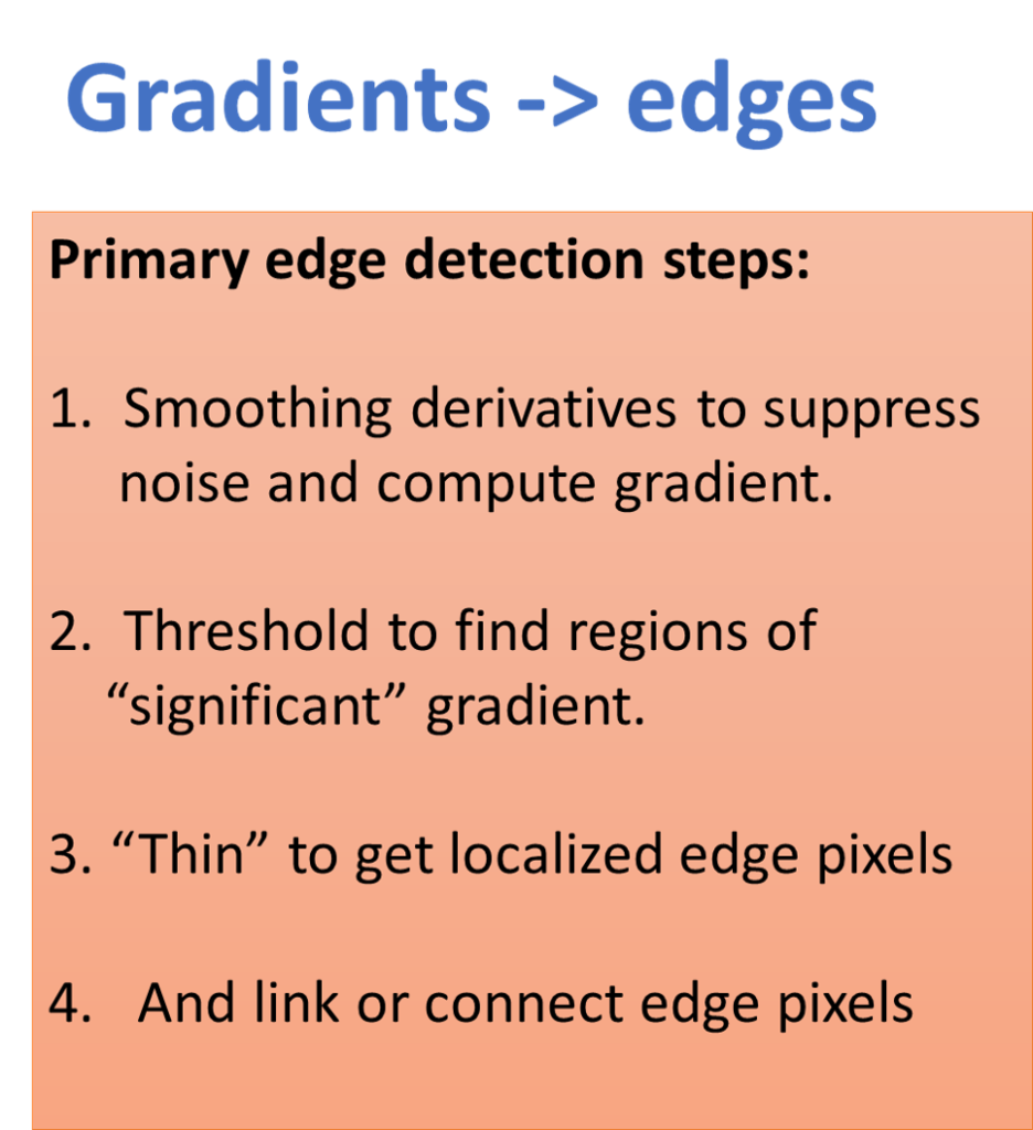
Let’s now get into this steps in a little more detail.
1. Smoothing derivatives and compute gradient
In the first step we are going to create smooth derivatives to suppress a little bit noise and we are going to compute the gradients. If we were to take just the magnitude of the gradient, we get a value that looks like this. You see it is close to edges, but actually, we can see edges. It is just a gradient image.

2. Thresholding
Next, we are going to

If we take a look, we will see that some of the pixels did not survive the thresholding. And it’s a problem because we can say we had too high a threshold. But the problem is if we make the threshold too low, then a whole bunch of stuff is going to show up that we don’t actually care about. So, the question is how to deal with that?
3. Thinning and Linking
Next we are going to take those areas and apply operation called thinning so that a fat edge becomes just a single contour. This is, in fact, non-maximal suppression. Basically saying if we have got a bunch of points that exceed a threshold locally, let us only pull out the point that exceeds it the most.
Finally, we need to connect those pixels to have a connected contour.
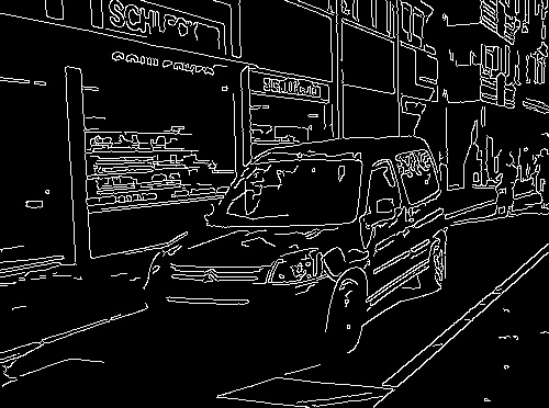
To sum up, the Canny operator works the following way: we first filter the image with the derivative of a Gaussian, we find the magnitude and orientation, then we do what is called non-maximum suppression, which is this thinning. And then, there is a linking operation where we are going to define not just one threshold, but two, and we are going to use the high threshold to start to edges, but we will use the lower threshold to continue.
Results
It is really hard to know when edges are good. It depends on for what are we going to use those edges. In general, the Canny Edge Operator gives us better edges that
4. Code for Canny Edge Detector:
Python
C++
#include <opencv2/opencv.hpp>
#include <iostream>

using namespace cv;
using namespace std;

int main()
{
    // Loading the actual image
    Mat image, gray, edges;

    image=imread("car.jpg", IMREAD_COLOR);

    // Edge cases
    if(image.empty()){
    	cout << "Error loading image" << endl;
    	return -1;
    }

    // converting the color image into grayscale
    cvtColor(image, gray, COLOR_BGR2GRAY);

    // Detect edges with Canny Edge Detector
    // First argument is the input image.
    // Second argument is the output image.
    // Third and fourth arguments are the minVal and maxVal.
    // Fifth argument is the size of Sobel kernel used for find image gradients (aperture_size).
    // Last argument is L2gradient.
    Canny(image, edges, 100, 200, 3);

    // Displaying the result
    cv::imshow("Original image", image);
    cv::imshow("Canny Edge Detector", edges);

    cv::waitKey(0);
    return 0;
}
Output:
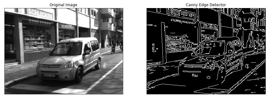
Obviously, this gives us much better results, as we can clearly see, edges are now more pronounced.
Summary
To summarize, we have learned how to use the Canny Edge Detector to detect edges, and how this algorithm works. In the next post, we will talk more about Hough transform and detecting lines.