Highlight: Welcome to another datahacker.rs post series! We are going to talk about digital image processing using OpenCV in Python. In this series, you will be introduced to the basic concepts of OpenCV and you will be able to start writing your first scripts in Python. Our first post will provide you with an introduction to the OpenCV library and some basic concepts that are necessary for building your computer vision applications. You will learn what images and pixels are and how we can access and manipulate them using OpenCV. So, without further ado, let’s begin with our lecture.

What is OpenCV?

OpenCV (Open Source Computer Vision Library) is an open source computer vision and machine learning software library that was built to provide a common infrastructure for computer vision, not to mention that the library has more than 2500 optimized algorithms! With this in mind, you can use it to detect and recognize faces, identify objects, classify human actions in videos, track movement with camera and many others.

Tutorial overview:

1. Introduction to the image basics
2. File extensions supported by OpenCV
3. What is a coordinate system?
4. Accessing and manipulating pixels in images with OpenCV
5. BGR color order in OpenCV
6. Funny hacking with OpenCV

1. Introduction to the image basics

What is a pixel?

The definition of an image is very simple: it is a two-dimensional view of a 3D world. Furthermore, a digital image is a numeric representation of a 2D image as a finite set of digital values. We call these values pixels and they collectively represent an image. Basically, a pixel is the smallest unit of a digital image (if we zoom in a picture, we can detect them as miniature rectangles close to each other) that can be displayed on a computer screen. 

A digital image is presented in your computer by a matrix of pixels. Each pixel of the image is stored an integer number. If we are dealing with a grayscale image, we are using numeric values from 0 (black pixels) up to 255 (white pixels). Any number in between these two is a shade of gray. On the other hand, color images are represented with three matrices. Each of those matrices represent one primary color which is also called a channel. The most common color model is the Red, Green, Blue (RGB). These three colors are mixed together to generate a broad range of colors. Note that OpenCV loads the color images in reverse order so that the blue channel is the first one, the green channel is the second, and the red channel is the third (BGR). 

To represent a single channel intensity values in an RGB image, we also use values from 0 to 255. Each channel produces a total of 256 discrete values, which corresponds to the total number of bits that you use to represent the color channel value \(2^{8}= 256 \). Since there are three different channels with 8 bits per channel, we call this a 24-bit color depth.

2. File extensions supported by OpenCV

So far, we have explained that the images in OpenCV are stored as matrices. However, one very important thing to note is that they are not necessarily stored, or transmitted in the same file format. Some file formats use different forms of compression to represent images more efficiently and they may not be supported by OpenCV.

In the following section, we will go over which of those file formats are supported by OpenCV.

1. Windows bitmap (bmp, dib)

The BMP file format, also known as bitmap image file or device independent bitmap (DIB), is a raster graphics image file format used to store bitmap digital images, independently of the display device. It is capable of storing two-dimensional digital images both monochrome and color, in various color depths, and optionally with data compression, alpha channels, and color profiles.

2. Netpbm – Portable image formats (pbm, pgm, ppm)

Netpbm is an open-source package of graphics programs and a programming library. Several graphics formats are used and defined by the Netpbm project. The portable pixmap format (PPM), the portable graymap format (PGM) and the portable bitmap format (PBM) are image file formats designed to be easily exchanged between platforms.

 3. Sun Raster (sr, ras)

Sun Raster was a raster graphics file format used on SunOS by Sun Microsystems. The format was mainly used in research papers.

4. JPEG (jpeg, jpg, jpe)

JPEG is a raster image file format that’s used to store images that have been compressed to store a lot of information into a small file. 

5. JPEG 2000 (jp2)

JPEG 2000 (JP2) is an image compression standard and coding system. It is a discrete wavelet transform (DWT) based compression standard that could be adapted for motion imaging video compression with the Motion JPEG 2000 extension. A standard uses wavelet based compression techniques, offering a high level of scalability and accessibility. In other words JPEG 2000 compresses images with fewer artifacts than a regular JPEG.

6. TIFF files (tiff, tif)

It is an adaptable file format for handling images and data within a single file.

7. Portable network graphics (png)

It is a raster-graphics file-format that supports lossless data compression. A PNG was developed as an improved, non-patented replacement for Graphics Interchange Format (GIF).

3. What is a coordinate system?

In the following example we see an image that is shown as a collection of pixels. If we want to asses a single pixel in the image, we will use a coordinate system. 

Pixels are accessed with two \((x, y) \) coordinates. The \(x \) value represents the columns and the \(y \) value represents the rows. As you can see in our example, the upper left corner of the image has the coordinates of the origin \((0, 0) \). Moreover, values for \(x \) coordinates increase as they go right and values for \(y \) coordinates increase as they go down.

It is important to note that NumPy always reads first the vertical values from the \(y \) axis, and then, the horizontal values from the \(x \) axis. Then, we will actually reverse the coordinates when we want to work with them as matrices both in OpenCV and NumPy.

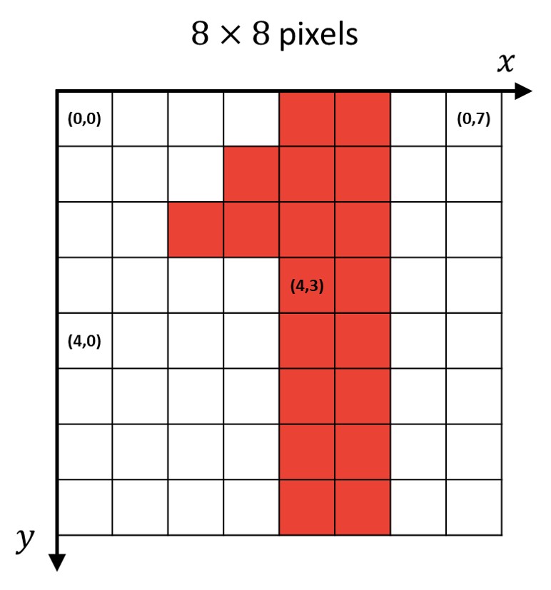
We can assess and manipulate each pixel in an image in a similar way: as an individual element of an array referenced in Python. Now, let’s see how we can do this with code.

4. Accessing and manipulating pixels in images with OpenCV

It is good to note that we are mainly going to use grayscale images as a default choice. Due to only one channel, it makes image processing more convenient. Usually, we convert an image into the grayscale one, because we are dealing with one color and it is a lot easier and faster. In OpenCV we can perform image and video analysis in full color as well, which we will also demonstrate.

Now, we are going to see how we can work with BGR images in OpenCV.

First, we need to read the image we want to work with using the cv2.imread() function. If the image is not in the working directory, make sure to know the exact file path. If we are working in Google Colab we need to upload our image from our computer. With this in mind, in the following examples we are going to read the image of the Tesla truck.

# Necessary imports
import cv2
import numpy as np
import matplotlib.pyplot as plt
# For Google Colab we use the cv2_imshow() function
from google.colab.patches import cv2_imshow

If we want to load a color image, we just need to add a second parameter. The value that’s needed for loading a color image is cv2.IMREAD_COLOR. There’s also another option for loading a color image: we can just put the number 1 instead cv2.IMREAD_COLOR and we will obtain the same output.

# Loading our image with a cv2.imread() function
img=cv2.imread("Cybertruck.jpg",cv2.IMREAD_COLOR)
# img=cv2.imread("Cybertruck.jpg",1)

The value that’s needed for loading a grayscale image is cv2.IMREAD_GRAYSCALE, or we can just put the number 0 instead as an argument.

# Loading our image with a cv2.imread() function
gray=cv2.imread("Cybertruck.jpg",cv2.IMREAD_GRAYSCALE)
# gray=cv2.imread("Cybertruck.jpg",0)

 To display an image, we will use the cv2.imshow() function.

# For Google Colab we use the cv2_imshow() function
# but we can use cv2.imshow() if we are programming on our computer 
cv2_imshow(img)
cv2_imshow(gray)

Output:

Our output for the grayscale image is the following:

Output:

Moreover, it is also possible to show images using the matplotlib library and the plt.imshow() function. Note, that here, we need to pay attention to the order of color channels. Let’s see!

# We can show the image using the matplotlib library. 
# OpenCV loads the color images in reverse order: 
# so it reads (R,G,B) like (B,G,R)
# So, we need to flip color order back to (R,G,B)
plt.imshow(cv2.cvtColor(img, cv2.COLOR_BGR2RGB))
# We can use comand plt.axis("off") to delete axis
# from our image
plt.title('Original')

Output:

After we load the image, some descriptors can be extracted from it:

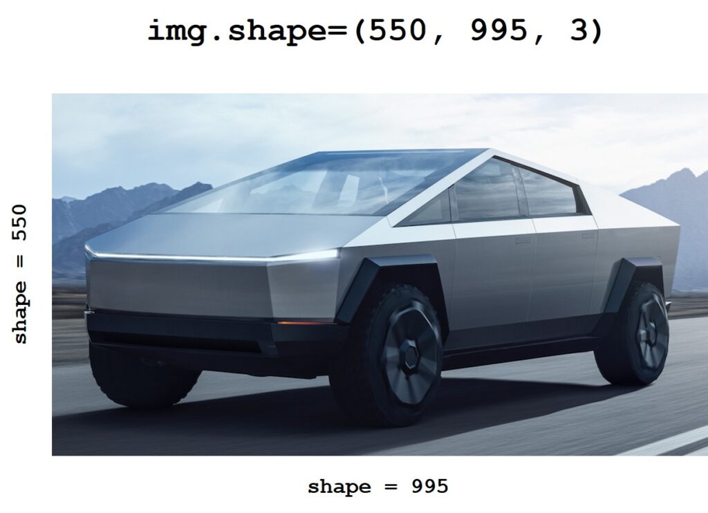
# If we want to get the dimensions of the image we use img.shape
# It will tell us the number of rows, columns, and channels 
dimensions = img.shape
print(dimensions)

Output:

(550, 995, 3)

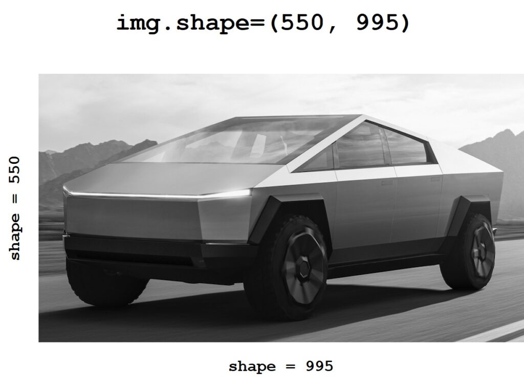
# If an image is a grayscale, img.shape returns 
#the number of rows and columns
dimensions = gray.shape
print(dimensions)

Output:

(550, 995)

# We can obtain a total number of elements by using img.size
total_number_of_elements= img.size
print(total_number_of_elements)

Output:

1641750

# Image data type is obtained by img.dtype
image_dtype = img.dtype
print(image_dtype)

Output:

uint8

Furthermore, we can access a pixel value by putting a row and a column coordinates and also store the color channels in a tuple.

# To get the value of the pixel (x=50, y=50), we would use the following code
(b, g, r) = img[50, 50]
print("Pixel at (50, 50) - Red: {}, Green: {}, Blue: {}".format(r,g,b))

Output:

Pixel at (50, 50) – Red: 210, Green: 228, Blue: 238

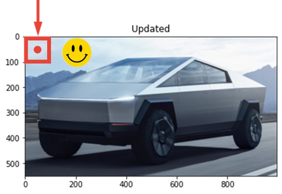
We can manipulate a pixel in the image, by updating the values into a new set of values

# We changed the pixel color to red
img[50, 50] = (0, 0, 255)

# Displaying updated image
plt.imshow(cv2.cvtColor(img, cv2.COLOR_BGR2RGB))
plt.title('Updated')

Output:

# Using indexing we modified a whole region rather than one pixel
# For the top-left corner of the image, we can rewrite 
# the color channels in folowing way:
img[0:150, 0:300] = [0,255,0]

cv2_imshow(img)

Output:

5. BGR color order in OpenCV

As we have already mentioned, OpenCV loads the color images in reverse order and uses the BGR color format instead of the RGB. We can see the order of the channels in the following diagram:

Due to this, we might have somewhat of a problem because other Python packages use the RGB color format, for example matplotlib. This is why it is very important to know how to convert an image from one format into another. Here is one way how it can be done in a fancy way.

# We load the image using the cv2.imread() function
# Function loads the image in BGR order
img3=cv2.imread("Pamela.jpg",1)
cv2_imshow(img3)

Output:

But when we are plot our image with matplotlib due to the fact that it uses RGB color order, colors in our displayed image will be reversed. See below.

plt.imshow(img3)

Output:

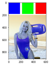
# We can split the our image into 3 three channels (b, g, r)
b, g, r = cv2.split(img3)

# Next, we merge the channels in order to build a new image 
img4 = cv2.merge([r, g, b])

Now, we have two images. The first one is our original image. In addition, we also created the second one (img2) where we split the original image into 3 channels and then merged them back together in RGB order. Next, we are going to plot both images, first with OpenCV and then with matplotlib. 

OpenCV:

cv2_imshow(img4)

Output:

Matplotlib:

plt.imshow(img4)

Output:

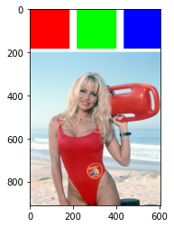
So, now, for img2, matplotlib works properly, but for the OpenCV we got a reversed colors. Luckily, it is easy for us visually to inspect whether the colors are displayed correctly.

6. Funny hacking with OpenCV

 For fun, let’s try and create our own images!

import numpy as np
gray = np.zeros( (256,256), dtype="uint8" )

for i in range(256):
  gray[i,:] = i
gray=gray.astype("uint8")
cv2_imshow(gray)

Output:

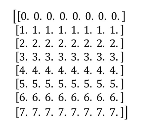
We created this grayscale transition along the \(y \) axis. As an experiment, we can print our image in \(8\times 8 \) resolution to show you the pixel values. You would get this output if in the previous code you replace 256 with 8.

print(gray)

Output:

We can do the same trick, and create this transition along the \(x \) axis.

for i in range((256)):
  gray[:,i] = i
gray=gray.astype("uint8")
cv2_imshow(gray)

Output:

Let’s now create the grayscale transitioning along diagonal of our image. We use int casting, as we need to convert it to an integer values, due to multiplication with 0.5.

for i in range(256):
  for j in range(256):
    gray[i,j]= (i*0.5 + j*0.5)

gray=gray.astype("uint8")
cv2_imshow(gray)

Output:

Okay, now let’s add some color:

r = np.zeros((256,256),dtype="uint8")
g = np.zeros((256,256),dtype="uint8")
b = np.zeros((256,256),dtype="uint8")

for i in range(256):
  for j in range(256):
    r[i,j]= i  
    g[i,j]= 0
    b[i,j]= 0

r=r.astype("uint8")
g=g.astype("uint8")
b=b.astype("uint8")

img = cv2.merge( (b,g,r) )    
cv2_imshow(img)

Output:

Or how about adding two colors?

r = np.zeros((256,256),dtype="uint8")
g = np.zeros((256,256),dtype="uint8")
b = np.zeros((256,256),dtype="uint8")

for i in range(256):
  for j in range(256):

    r[i,j]= (i*0.5 + j*0.5)
    g[i,j]= j
    b[i,j]= 0

r=r.astype("uint8")
g=g.astype("uint8")
b=b.astype("uint8")

img = cv2.merge( (b,g,r) )    
cv2_imshow(img)

Output:

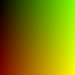
This should be enough 🙂 You get an idea how creative you can be with pixels and for loops!

Summary

In this post we covered some key concepts related to images. To sum it up, we have learned that OpenCV uses the BGR color format instead of RGB. We have learned what pixels are and how to access and manipulate them in Python. In addition, we have explained how to create new images and how to index them. In the next post we will see how to work with videos using OpenCV.

References:

[1] Intro and loading Images – OpenCV with Python for Image and Video Analysis 1