CamCal #000 Perspective Imaging
Perspective Imaging
Highlights: In this post we’re going to talk about perspective imaging. First, there is a little bit of math that is needed for the explanations of the geometry and the configuration of the camera. Second, we will use a simplified pinhole camera model. Hence, we will not talk about focus and other “non-pinhole effects” when the rays are not in focus.
When we take a photo, our 3D world is mapped into a 2D image. This post explains how we can better understand and model this process.
Tutorial Overview:
1. Coordinate system
Once we take a photo or a selfie with our camera, we actually go from 3D to 2D world. Formally speaking, this process is called a projection and is commonly used in linear algebra. Why do we need such a projection model, you can ask yourself?
Well, suppose that you take an image in Paris and ask yourself how tall the Eiffel tower is? The projection modeling can assist us to solve this task using computer vision methods.
Therefore, before we derive a model for a projection step, we will have to refresh our knowledge about coordinate systems.
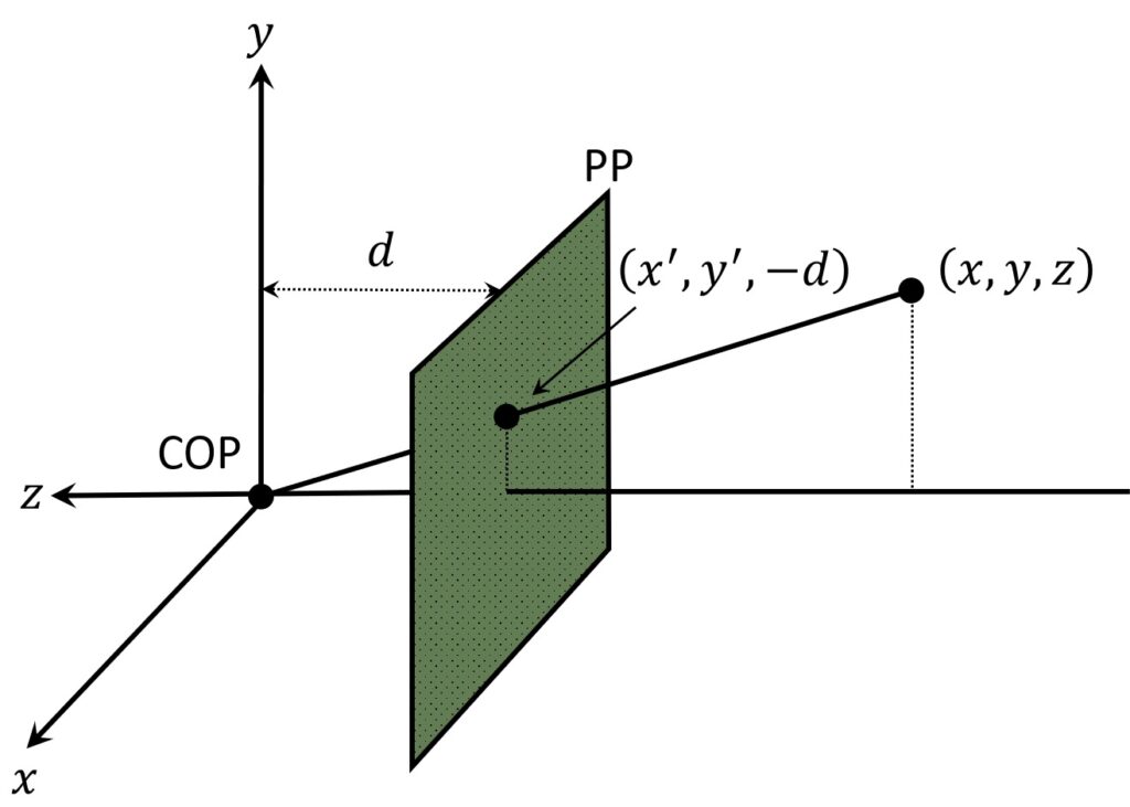
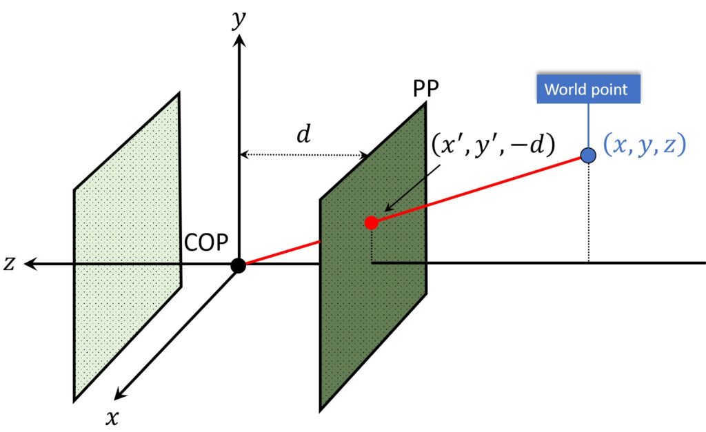
In the image above, we have a coordinate system and we will use it for our camera pinhole model. First, we can see that the origin of the coordinate system is located at the center of projection (COP). Second, this center, also represents the origin of our camera coordinate system as well.
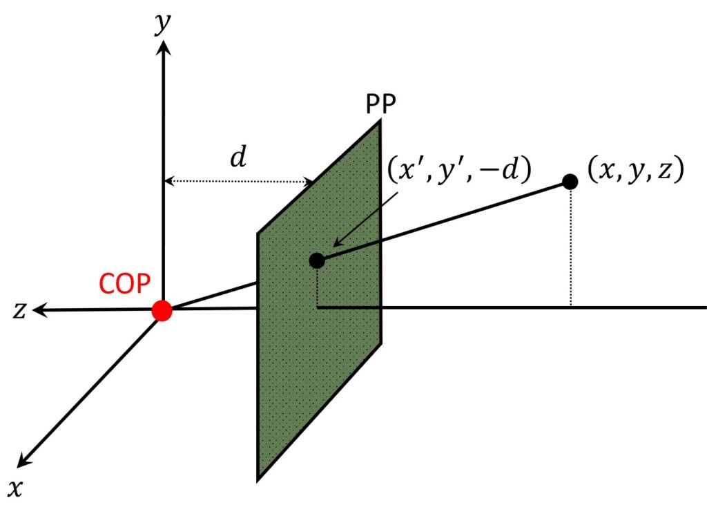
Along with our center of projection (COP), we’re also going to use a standard \(\left ( x,y \right ) \) coordinate system to specify the objects. So \(\left ( x,y \right ) \) are like regular axis coordinates. If we imagine that we look exactly from the COP, \(x \) will go to the right and \(y \) will go into upward direction.
Next, we will apply something a little bit different than commonly used. The COP represents a pinhole and once a light passes through it, an image will be formed behind it. However, this image will actually be inverted. That is, image axes will be flipped when compared with 3D axes. So, due to mathematical convenience, we will imagine that the image is somehow formed in front of the pinhole. In this way, our image will be neither inverted nor flipped. This will make our analysis easier, without loss of generality.
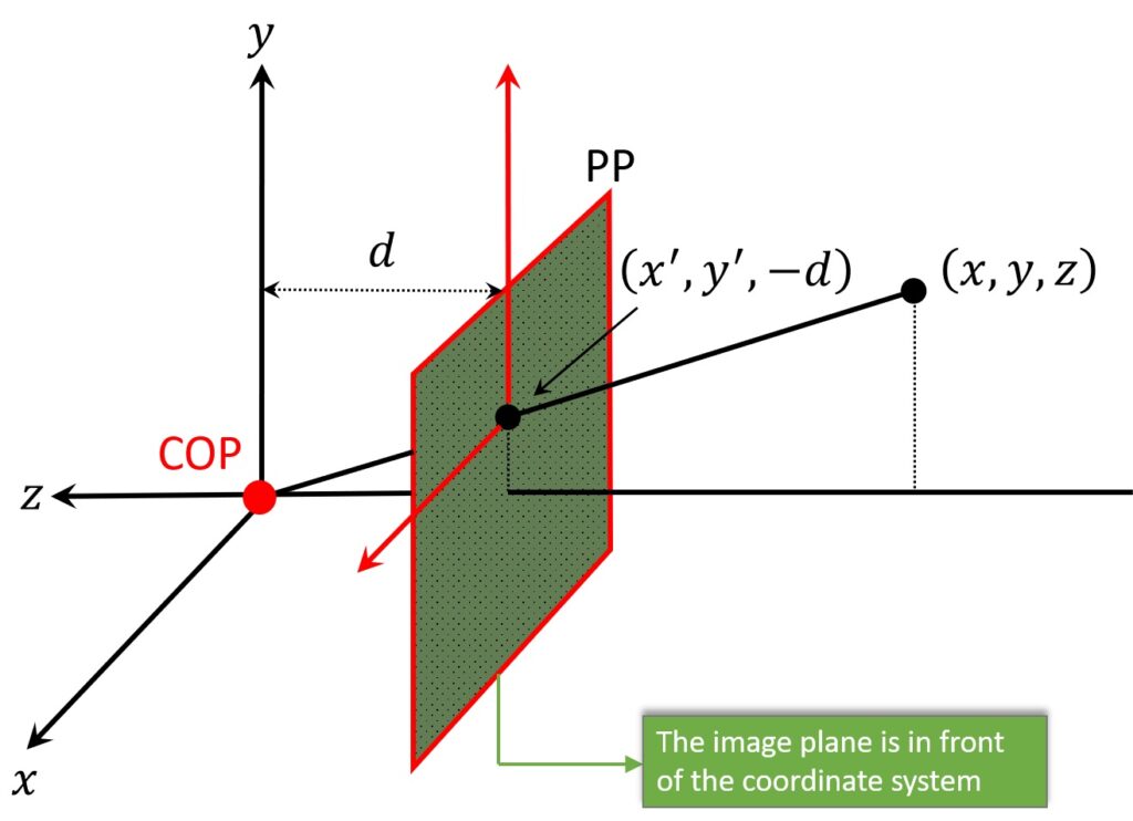
Further, one of the implications of this \(\left ( x,y \right ) \) coordinate system, in order for this to remain a right-handed coordinate system, \(z \) is now pointing from the camera, not out to the world. Note that this is marked in Figure below with red.
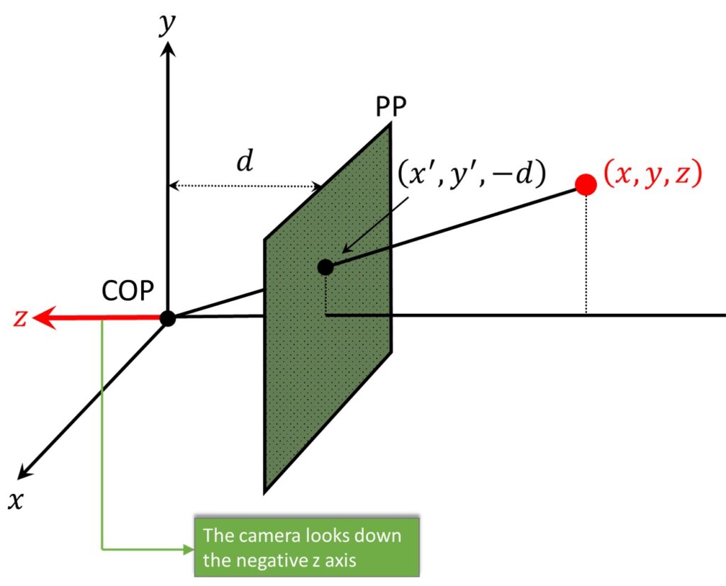
The direction of the \(z \) axis is not of such a great importance. For instance, we wrote down that the world’s position of some point was \(\left ( x,y,z \right ) \). We didn’t explicitly say negative \(z \) because it’s a \(z \) value. This value can, of course, be a negative 20.
In order to better illustrate this, let’s again have a look at our world point. The ray passes through it down to the center of projection. Hence, normally our image plane would be behind COP (light green plane). Here, the idea is that, the ray intersects the image plane at this point (marked in red), which we’re going to call \(\left ( {x}’,{y}’ \right ) \). We will write \(–d \) because the focal length distance \(d \) from the COP to the image plane, is a positive distance. In this way, the location of this point is going to be \(\left ( {x}’,{y}’,-d \right ) \).
2. Modeling Projection
In the following text, we will use the projection of the world point onto the image plane to derive the projection equations. It is interesting to have a look at this intersection point of the ray and a projection plane. This is a point \(\left ( {x}’,{y}’ \right ) \), and we can connect this point to \(z \) axis. Next, we can notice the appearance of two similar triangles, colored in red and green.
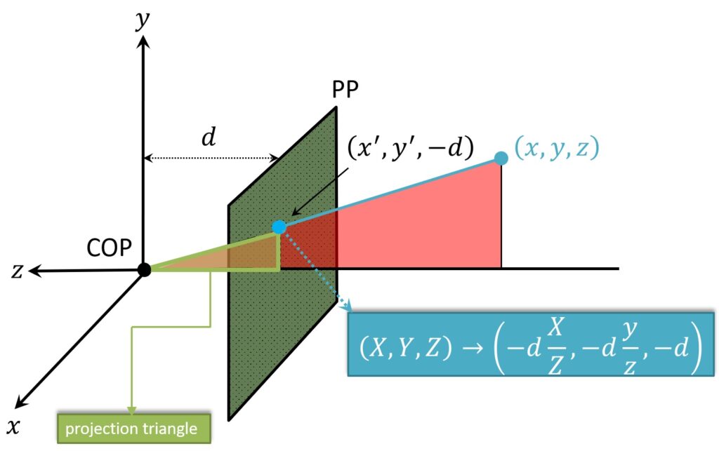
Using the similarity properties of the triangles, we get that the \(\left ( x,y,z \right ) \) location, the location of the world point, is now mapped into the point in the image plane: \(\left ( -d\frac{X}{Z},-d\frac{Y}{Z},-d \right ) \).
So, the derived Projection equations are:
$$ \left ( X,Y,Z \right )\rightarrow \left ( -d\frac{X}{Z},-d\frac{Y}{Z},-d \right ) $$
The projection formula simply divides all the coordinates with the value of a coordinate \(Z \) and multiply it with the negative focal length \(d \). We need one additional step to get the location of the intersection point in the coordinate of the image itself. This step, is fairly simple and we just omit the \(Z \) coordinate. Hence the new image coordinates are going to be:
$$ \left ( {x}’,{y}’ \right )= \left (-d\frac{X}{Z},-d\frac{Y}{Z} \right ) $$
One of the obvious implications of a division by \(Z \) is that farther objects will appear smaller in the image. Naturally, this is something that we know from our everyday experience. If we take an object and pull it further away, its size in the image gets smaller. This is because we’re doing perspective projection and the points are mapped to the values that are proportional to \(\frac{X}{Z} \) and \(\frac{Y}{Z} \).
3. Homogeneous coordinates
Previously, we have described the process of mapping the coordinates by doing the following divisions: \(\frac{X}{Z} \) and, \(\frac{Y}{Z} \). Now, the question is whether this is a linear transformation? The answer is obvious. No. Well, for sure a division itself is a linear operation. For example, a division by some constant \(\frac{1}{a} \) is a linear operation. However, here we have \(\left ( x,y,z \right ) \), and we actually have to pull out that \(z \) and divide the \(x \) and the \(y\) by it. And so, if we’ve got another point with \(\left ( x_{1},y_{1},z_{1} \right ) \), we divide by that \(z_1 \). That is why it’s not a linear operation, and we have to essentially change what’s going on. So, now we are going to do a trick. And the trick is, we are going to add one more coordinate. We can do this in either two dimensions or three dimensions.
In two dimensions:
$$ \left ( x,y \right )\Rightarrow \begin{bmatrix} x\\ y\\ 1\end{bmatrix} $$
It three dimensions:
$$ \left ( x,y,z \right )\Rightarrow \begin{bmatrix}
x\\
y\\
z\\
1\end{bmatrix} $$
And this bottom coordinate, which right now here is written as a 1, that’s the homogeneous coordinate or the homogeneous component of the vector.
So, converting from regular coordinates to homogenous and back again is pretty easy. If we have the homogeneous coordinate:
$$ \begin{bmatrix}x\\y\\w\end{bmatrix}\Rightarrow \left ( x/w,y/w \right ) $$
We get the nonhomogeneous by just dividing by \(w \). And for 3D we have
\(x \), \(y \), and \(z \), each over \(w \):
$$ \begin{bmatrix}x\\y\\z\\w\end{bmatrix}\Rightarrow \left ( x/w,y/w,z/w \right ) $$
Now we can see why converting \(\begin{bmatrix}x\\y\\1\end{bmatrix}\) to nonhomogeneous, we still get back the \(x \) and \(y \) as we had before. But if that last homogenous coordinate is not 1, then we’ll get a different value. By the way, this makes homogeneous coordinates invariant under scale. If we were to multiply the entire homogeneous coordinate by some constant, \(a \). So, we have:
$$ \begin{bmatrix}ax\\ay\\aw\end{bmatrix} $$
When we do the conversion back again doing the division, the \(a \) will cancel out.
Summary
To summarize, we have learned how to model a projection, and what are homogeneous coordinates . In the next post, we will talk more about Perspective Projection and Vanishing Points.