#017 CNN Inception Network

\(Inception\enspace network \)
Motivation for the \(Inception\enspace network \):
In the last post we talked about why \(1\times 1 \) convolutional layer can be useful and now we will use it for building the \(Inception\enspace network \).
When designing a layer for a \(convnet \) we might have to choose between a \(1 \times 3 \) filter, a \(3 \times 3\) or \(5\times 5\) or maybe a pooling layer. An \(Inception\enspace network \) solves this by saying:“ Why shouldn’t we apply them all ? ”. This makes the network architecture more complicated, but remarkably improves performance as well. Let’s see how this works.

An \( Inception \enspace network \) architecture
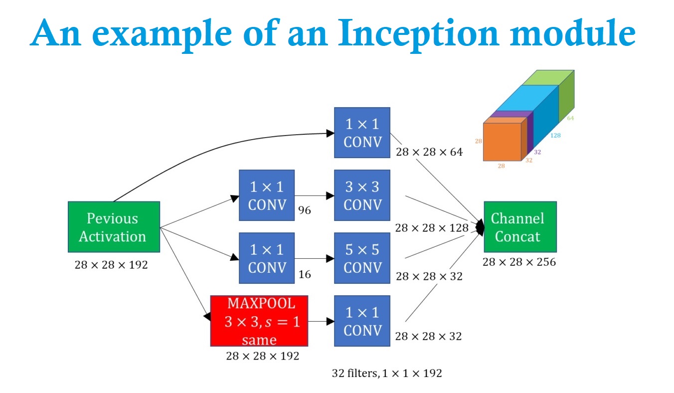
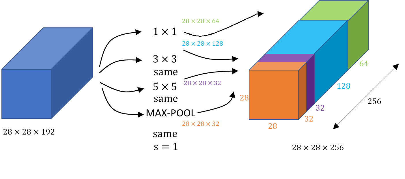
Suppose that we have an input that is \(28\times28\times 192 \) dimensional volume. Commonly, we will have to decide if we are going to apply \(conv \) layer or a \(pooling\enspace layer \). In case that we choose the \(pooling\enspace layer\), we will have to choose the filter size. Surprisingly, the \(Inception\enspace network \) solves this in a very elegant way. In this example, we can apply \(1 \times 1 \) convolution using \(64 \) filters and that will output a \(28 \times 28 \times 64 \) volume. In addition, let’s also apply \(128 \enspace 3\times3 \) filters, and this will obtain \(28\times28\times128 \) volume. Then, we will just stack these two outputs next to each other. Subsequently, we will repeat the similar process with different filters.
The \(Inception\enspace network \) or an inception layer says: instead of choosing the desired filter size in a \(conv \) layer or whether we want a \(convolutional \) layer or a \(pooling \) layer, let’s apply all of them.
If we use a \(1 \times 1\) convolution that will output a \(28 \times 28 \times 64\) output ( a green volume on the picture above). If we also want to try a \(3 \times 3 \) filter that will output a \(28\times28\times128 \) volume (a blue volume). Next, we just stack up the second volume next to the first volume. To make the dimensions match up. Let’s make this a \(same \) convolution so the output dimension is still \(28 \times 28\), that is, same as the input dimension in terms of height and width. We may also add a \(5\times 5\) filter, and this will create a \(28\times28\times 32 \) output. We again use the same convolution to keep the dimensions the same. Let’s apply pooling, and here pooling outputs \(28\times28\times 32 \) (orange volume) . In order to make all the dimensions match we actually need to use padding for Max pooling. This is an unusual form of polling because if we want the input to have higher worth than \(28 \times 28 \) and have the output that match the dimension everything else also by \(28 \times 28\). Then we need to use same padding as well as the stride of \(1 \) for pooling. But with an inception module like this we can input some volume and output in this case \(32+32+128+64=256 \). So, we will have \(1 \) Inception module which has as an input \(28\times28\times128 \) volume and \(28\times28\times 256 \) dimensional volume as an output.
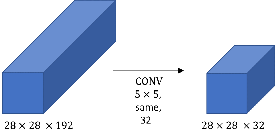
However, it turns out that there’s a problem with the inception layer and that is a computational cost. Let’s figure out what’s the computational cost of this \(5\times 5\) filter. We have as input a \(28\times28\times 192 \) block and we implemented a \(5\times 5\) same convolution or \(32 \) filters to output \(28\times28\times 32 \).
The problem of the computational cost
 Calculating the cost for to output the \(28\times 28 \times 32\) volume when the input volume is \(28\times 28 \times 192\) dimensions
In the previous image we had drawn this as a thin purple slice and we now just draw this as a blue block. Let’s look at a computational cost of generating a \(28\times28\times 32 \). We have \(32 \) filters because we want the output to have 32 channels. So each filter that we are going to use will be \(5\times 5\times192\).
The output size is \(28\times28\times 32 \) so we need to compute \(28\times28\times 32 \) numbers and for each of them we need to do \(5\times 5\times192\) multiplications . The total number of multiplications we need is the number of multiplications we need to compute each of the output values times the number of output values we need to compute. And if we multiply out all these numbers this is equal to \(120 \) million.
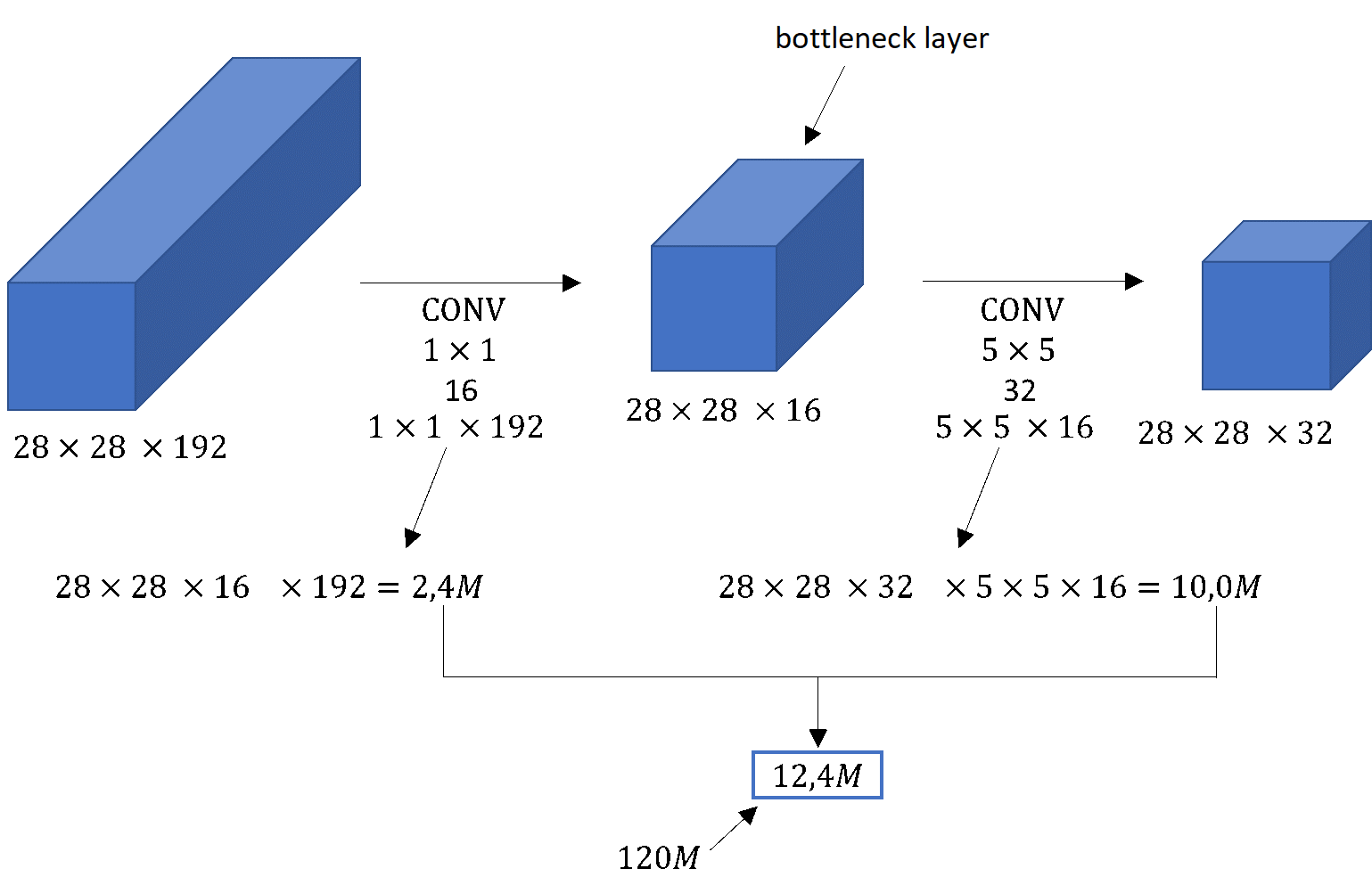
While we can do \(120 \) million multiplies on the modern computer this is still a pretty expensive operation. On the next line we see how using the idea of \(1 \times 1 \) convolutions, which we learned in the previous lecture, we’d be able to reduce the computational cost by about a factor of \(10 \), to go from about \(120 \) million multiplications to about 1/10 of that. Remember the number \(120 \) million so that we can compare it with what we see on the next slide. Here’s an alternative architecture for inputing \(28\times28\times 192 \) and outputting to an \(28\times28\times 32 \).
We’re going to use a \(1 \times 1 \) convolution to reduce the volume to a \(16 \) channels instead of \(192 \) channels. Then on this much smaller volume we will apply our \(5\times 5\) convolution to give us our final output. Notice that the input and output dimensions are still the same. We input \(28\times28\times192 \) and output \(28\times28\times 32 \) same as the previous example. Here, by use of \(1\times1 \) convolution, we shrunk the big volume on the left, obtaining in this way \(16 \) instead of \(192 \) channels.
Using 1x 1 convolution

Comparation of number of elements to be learned
Now let’s look at the computational cost. To apply this \(1 \times 1 \) convolution we have \(16 \) filters. Each of the filters is going to be of dimension \(1 \times 1 \times 192 \). The cost of computing this \(28 \times 28 \times 16 \) volume is going to equal to the number of computations and it’s \(192 \) multiplications.
The cost of this first convolutional layer is learning about \(2.4 \) million parameters. The cost of the second convolutional layer will be about \(10.0 \) million because we have to apply \(5\times 5 \times 16 \) dimensional filter on this \(28\times 28\times 32 \) dimensional volume above.
So, the total number of multiplications we need to do is the sum of those, which is \(12.4 \) million multiplications. If we compare this with previous example we reduced the computational cost from about \(120 \) million multiplications down to about 1/10 of that, to \(12.4 \) million multiplications. The number of additions we need to perform is very similar to the number of multiplications as well.
In case that we’re building a layer of a neural network and we cannot decide what layer to use the inception module says let’s do them all and let’s concatenate the results. Then we ran into the problem of a computational cost. What we saw here was how using a \(1 \times 1 \) convolution we can create a bottleneck layer, thereby reducing the computational cost significantly. You might be wondering, does shrinking down the representation size so dramatic, it hurts the performance of our neural network. It turns out that as long as we implement this bottleneck layer so the proven reason, we can shrink down the representation size significantly and it doesn’t seem to decrease the performance, but saves us a lot of computation. These are the key ideas of the inception module. Let’s put them together and in the next post we’ll see what the full \(Inception\enspace network \) looks like.