#012 Blending and Pasting Images Using OpenCV
Highlights: Often, we come across projects or tasks where we need to merge or mix two images. However, due to various parametric restrictions such as sizing, the task seems difficult to execute. Also, it can be boring when it is done in Photoshop. However, this process can be quite interesting if it is fully automated.
In this post, we will make the blending and pasting of images on top of each other, fun and interesting. We will work with multiple images of varying parameters and learn how to conduct the blending and pasting process on those images using an OpenCV program.
Tutorial Overview:
- Introduction to Blending and Pasting
- Blending Images of Same Sizes with OpenCV
- Blending Images of Different Sizes
1. Introduction to Blending and Pasting
Blending and pasting is used commonly to mix two images or overlay an image on top of another image. There are many applications for blending and pasting such as graphic designing, logo placement, internet meme generation. All of these applications can be easily and quickly processed using OpenCV.
In order to understand the blending and pasting process, we need to learn several different methods in OpenCV programming.
The image pasting is a process of overlaying one image on top of the other. To successfully apply this process in OpenCV we need to select Region of Interest (ROI) in the first image, and then apply masking and some logical operations to overlay second image over the first image.
The process of blending s done through the cv2.addWeighted() function from OpenCV. This function uses both the input images, assigns certain weights to each image pixel, adds them together and outputs the result into a new pixel. In that way we will get the us an impression of transparency. In the following example you can see the difference between pasting one image on top of other and blending two images together.

The formula for this operation can be written as:
$$ p=\alpha p_{1}+\beta p_{2}+\gamma $$
In the following image, blending operation with the cv2.addWeighted() function is illustrated.

The output pixel \(p \) in the new blended image is equal to the sum of three parameters. First we have the parameter \(\alpha \), which is a weight multiplied with the pixel in the first image. Then, we add this to another parameter \(\beta \) which is a weight multiplied with the pixel in the second image, at the same location as the pixel in the first image. We can also add another factor \(\gamma \) as an option and calculate the total weighted sum using the expression above.
So, if we want Pixel 1 from the first image to be more pronounce, we could simply increase the value of \(\alpha \). Similarly, if we want Pixel 2 from the second image to be less represented in the blended version, we could just decrease our \(\beta \) value.
Thus, choosing the right values for \(\alpha \) and \(\beta \) can affect which image will show up stronger or weaker in the output blended image. Additionally, the factor \(\gamma \) can be used to manipulate the image further, according to specific requirements.
The process of image blending is much simpler when the two input images are of same size. However, the same process gets slightly more complicated when these two input images are of different sizes. In the upcoming sections of this tutorial post, we will see how we can blend and paste images on top of each other under both circumstances. So, let’s begin.
2. Blending Images of Same Sizes with OpenCV
To start with, we will import all necessary libraries. Next, we will open all images that we’re going to work with.
# Necessary imports
import numpy as np
import cv2
import matplotlib.pyplot as plt
from google.colab.patches import cv2_imshow
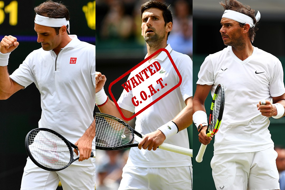
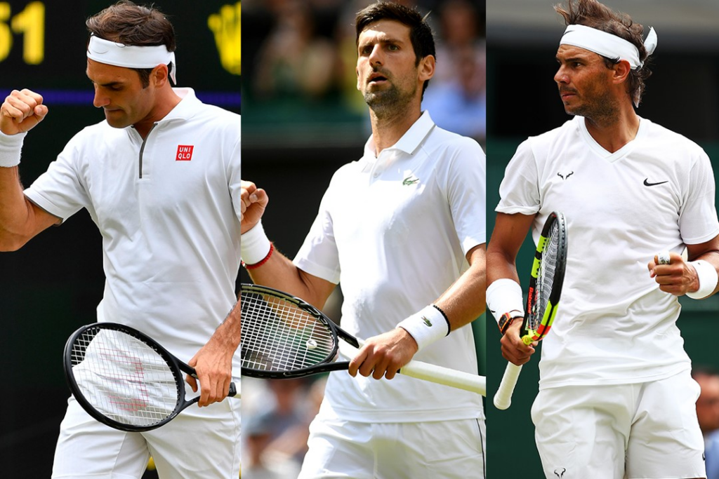
In our example, the first image is going to be the picture of three greatest tennis players of all time: Roger Federer, Rafael Nadal and Novak Djokovic. The second image is going to be what’s known as a watermark.
large_img = cv2.imread('FDN.jpg')
watermark = cv2.imread('Watermark.jpg')cv2_imshow(large_img)Output:
cv2_imshow(watermark)Output:

As you can see, we have imported and opened our images. We can, now, check the shapes of these images and see if both our images are of the same sizes. Currently, the images are not of the same size, so we will need to do a bit of resizing.
print (large_img.shape)
print (watermark.shape)
Output:
((720, 1080, 3)
(480, 640, 3)
The resizing of images is done such that both the images are of exactly the same size. Here, we will maintain a common size for the images as \(800 \times600 \). Note, that this will result in a slight distortion of our images. Ideally, we would want to create a mask here, but to keep it simple for our first example, we will go ahead as it is with distorted images. We will tackle the issue of different image sizes when it comes to blending, in a separate section, ahead in our blog post.
We will resize the images using the function cv2.resize() as shown below.
img1 = cv2.resize(large_img,(800,600))
img2 = cv2.resize(watermark,(800,600))cv2_imshow(img1)Output:

cv2_imshow(img2)Output:

Now that we have resized our images, let’s get straight into blending them together.
As mentioned earlier in this post, we will use the function cv2.addWeighted(). Here, we will adjust a few parameters according to the equation we discussed above. In this case we will use the value of 0.5 for parameters \(\alpha \) and \(\beta \) and we will ignore the \(\gamma \) factor.
blended = cv2.addWeighted(img1, 0.5, img2, 0.5, 0)
cv2_imshow(blended)
Output:
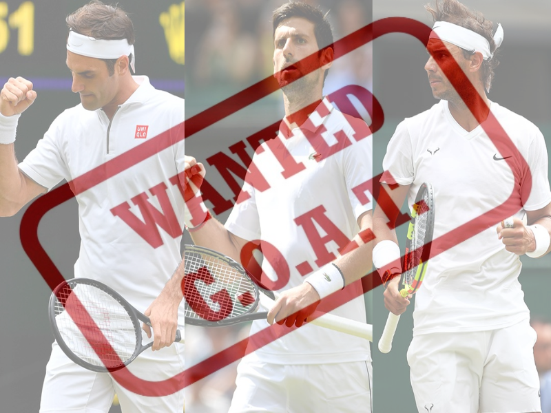
Observe the above result. Since \(\alpha \) and \(\beta \) values were the same, both images are equally represented in the result. Notice that the “Wanted G.O.A.T.” image has a white color as a background. Overlaying or blending this white background image on top of the first image makes the “Federer – Nadal – Djokovic” image a little faded.
Now, what if we wanted the first image to shine more? We will simply pass a much higher \(\alpha \) value and a much lower \(\beta \) value. Have a look at the result of this change below.
blended = cv2.addWeighted(img1, 0.8, img2, 0.2, 0)
cv2_imshow(blended)
Output:
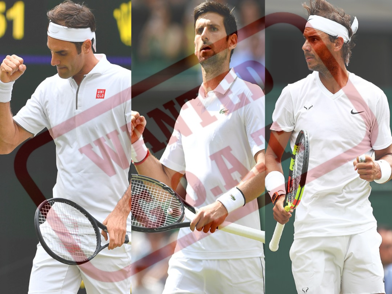
Notice how, now, we can only barely see the second image of the “Wanted G.O.A.T.” sign on top of our original “Federer – Nadal – Djokovic” image. This shows that manipulating the blending of two images is actually quite easy with the adjustment of \(\alpha \) and \(\beta \) values, respectively. Note, that if we use the value of 1 for \(\alpha \) and \(\beta \), the original pixel values will be added together.
blended = cv2.addWeighted(img1, 1, img2, 1, 0)
cv2_imshow(blended)
Output:

Also, note that if \(\gamma \) is equal to 255 all pixels in the output image will be white. You can also try experimenting on your own with the \(\gamma \) factor and see how it affects the output blend.
Let us now move ahead and blend two images of different sizes.
3. Blending Images of Different Sizes
In real life, we are not as lucky as in the previous example where we saw two images that have exactly the same size or can be resized equally without significantly distorting any image. If we were to try the same process as above with images of different sizes, we would get an undesired result. So, how do we tackle image blending when it comes to varying image sizes? Let’s use the same example images as above to demonstrate this.
The first operation we’ll perform is to make it appear like an overlay of a smaller image over the larger image. We won’t be performing blending for now. This operation is called pasting and it is performed using a NumPy reassignment operator. We will simply take the values of the larger image and reassign them to match the smaller image in a particular section of the larger image.
The second operation is where we will actually blend the images together. However, we won’t be using the cv2.addWeighted() function for that since it only works with images of same sizes. Instead we will create a mask using logical bitwise operations.
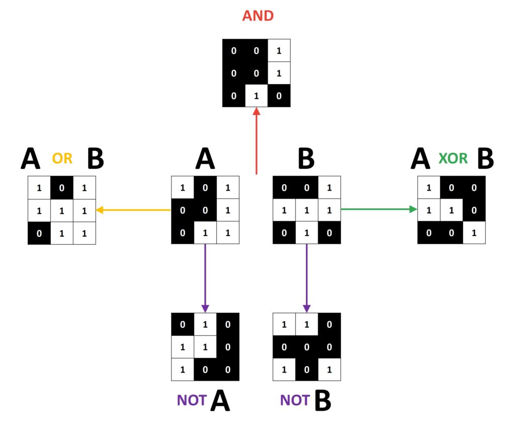
We use logical bitwise operations when we want to manipulate the values of the image for comparisons and calculations. There are four of these operations and they are very simple, and easy to understand.
- AND – True if both pixels are greater than zero
- OR – True if either of the two pixels are greater than zero
- XOR – True if either of the two pixels are greater than zero, but not both
- NOT – Invert pixel values
Overlaying Without Blending – pasting
The first operation that we will apply is the image pasting. Here, we won’t see the original image underneath the top image. So, let’s reload our images.
large_img = cv2.imread('FDN.jpg')
watermark = cv2.imread('Watermark.jpg')
To illustrate this section of blending images of varying sizes, we will make the second image a lot smaller so that there is a clear difference in size. Let’s resize it to, say, \(300\times300 \).
small_img = cv2.resize(watermark,(300,300))
cv2_imshow(small_img)
Output:
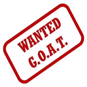
The larger image is of dimensions \(1080\times720 \), which means, the smaller image of dimensions \(300\times300 \) can easily be fit anywhere over the larger one.
Now, we need to figure out the actual logic of taking a chunk of the larger image pixel values and replacing them with the entire content of the smaller image. Well, it’s actually pretty straightforward process which is illustrated in the following image.

All you need to do is to define x_offset and y_offset. These are just going to stand as markers for where you actually start the image and where you’re actually going to overlay the image. In this case, we want to put “Wanted G.O.A.T.” over Roger Federer. That is why we set our x_offset and y_offset to 30 and 170 . Then, later on, we’ll play around with these values.
x_offset = 30
y_offset = 170
Now, we have got our x_offset and y_offset, but we need to define x_end and y_end as well. Here, x_end is essentially the offset plus the length of the smaller image. We can grab the shape of the small image, which returns a tuple. Here, we need a width of the small image and that is the second number in the tuple. Then, for y_end, we will write the same code but we will use the first number in the tuple which is the height of the small image.
x_end = x_offset + small_img.shape[1]
y_end = y_offset + small_img.shape[0]
Finally, all we need to do is to take the larger image, grab some chunk of \(x \) and some chunk of \(y \), and reassign it to be equal to the smaller image. So in this case, we want the larger image to be from the y_offset sliced all the way to y_end and the x_offset sliced all the way to the x_end. Let’s run that.
large_img[y_offset:y_end,x_offset:x_end] = small_img
cv2_imshow(large_img)
Output:
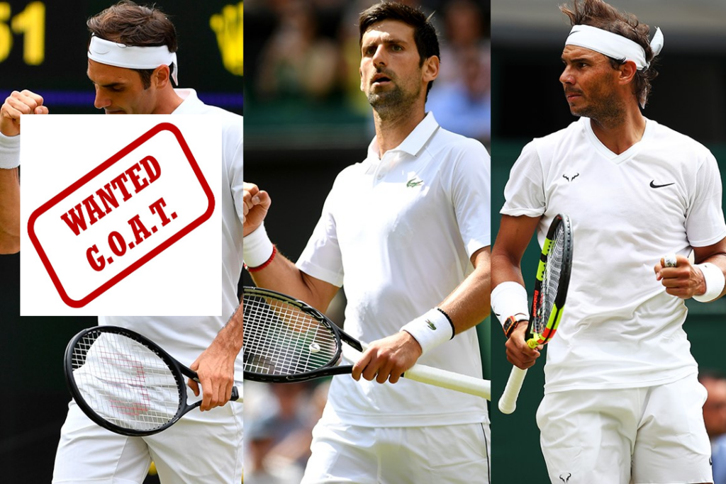
As you can see we have successfully overlaid the smaller image over the large one. Now, we will proceed to the second operation of actually blending images of different sizes over each other.
Blending Operation
Now, we learn how to blend images of different sizes. We need to select an ROI (Region Of Interest) in the first image, replace the values in that particular region with the values of the second image and then add them back in. However, the white background of the second image is quite annoying and our goal is to make only the logo visible. To do this we need to perform several masking procedures and bitwise operations.
To better understand this, let’s take a look at another example. On the left hand side, we can the image which is completely blue. The second image is the black image with red square in the middle. Now, notice what will happen if we apply the function cv2.addWeighted() using the equal values for \(\alpha \) and \(\beta \), and value of 0 for \(\gamma \). We can see that the values of the foreground and the background areas are blended according to the values of the \(\alpha \) and \(\beta \). That is why we can’t use the cv2.addWeighted() function for our purpose because we simply can’t chose the proper values for \(\alpha \) and \(\beta \) and \(\gamma \).

What we really want to achieve as a result is that the watermark appears without any background reference on top of the larger image, and that red color of letters in the watermark do not get blended with the pixels in the large image. In the following graph we illustrated all necessary steps that we need to apply in order to achieve our goal.

The entire process of blending images of different sizes involves three essential stages:
- Selecting image that needs to be pasted on a larger image.
- Building a mask to let only certain parts of the larger image to filter through to the next stage.
- Building another mask to let only certain parts of the smaller image to filter through to the next stage.
- Overlaying the masked image onto the larger image.
So, now we will see how we can actually create these masks in order to allow only certain parts of the smaller to pass onto the larger image.
As we did earlier, we will reload our images, the ones we used in previous sections as examples. Next, we will run the resizing command as shown below.
large_img = cv2.imread('FDN.jpg')
watermark = cv2.imread('Watermark.jpg')
small_img = cv2.resize(watermark,(300,300))
cv2_imshow(small_img)The next logical step is to decide where on the larger image do we need to place the smaller image. For this, we need to identify a suitable space of dimension \(300\times 300 \), on the larger. This will be our ROI (Region Of Interest).
In the previous section example, we chose the top left corner. Now, we want to place watermark across the tennis player who is the G.O.A.T..
Now, if we check the shape of the large image, we can see that the width is equal to 1080 and height is equal to 720. This means that we need to figure out our starting x_offset and our starting y_offset, respectively. We can do that simply by saying that x_offset is equal to 400 and y_offset is equal to 170. These are coordinates of the top left corner of the ROI.
x_offset = 400
y_offset = 170
Now, we need to create an ROI of the same size of the foreground image. The foreground image is nothing but the smaller image which will be placed on the top. We can use a tuple unpacking to reassign this by making the rows, columns, and channels equal to that of the image shape. In this way, we have generalized terms of rows as 300 and columns as 300, along with three color channels.
rows,columns,chanels = small_img.shape
roi = large_img[y_offset:470, x_offset:700]
Similar to what we did previously, we will grab the ROI by starting at y_offset=170 and then adding a 300 which is the y-axis coordinate of a small image (170+300=470). Then, we will start from our x_offset and do the same thing (400+300=700). Now, we can show our ROI. Notice how it is placed somewhere around Novak Djokovic, who is in our opinion the G.O.A.T.
cv2_imshow(roi)Output:
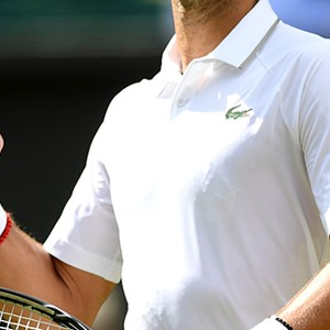
The next step is to create the mask for the smaller image such that we filter out everything except the red portion of the “Wanted G.O.A.T.” image. For this, we will first create a grayscale version of the image.
small_img_gray = cv2.cvtColor(small_img, cv2.COLOR_RGB2GRAY)
cv2_imshow(small_img_gray)
Output:

Notice that letters in this image are not exactly colored in black but rather in some dark gray color. That is why we need to apply a thresholding in order to create a binary image.
ret, mask = cv2.threshold(small_img_gray, 120, 255, cv2.THRESH_BINARY)
cv2_imshow(mask)
Output:
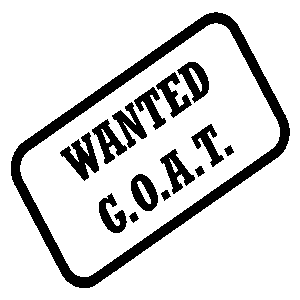
That is our mask. Now, we will apply a cv2.bitwise_or operation. As parameters we will pass the ROI and the mask into this operator. In that way we will create our bedground.
bg = cv2.bitwise_or(roi,roi,mask = mask)
cv2_imshow(bg)
Output:
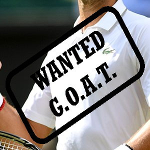
For the foreground we need to create black image with the red watermark. In order to bring back the red color, we need to inverse the mask. We can do that by using the cv2.bitwise_not operation, which will calculate the per-element, bitwise inversion of the input image. This means that this operator will convert everything black into all white and everything white into all black.
mask_inv = cv2.bitwise_not(small_img_gray)
cv2_imshow(mask_inv)
Output:

Notice the result above. We can see the inverted image, where the white space is, will allow anything to shine through. In our case, we want it to shine ‘red’. For that we will use the cv2.bitwise_and function and as parameters we will pass small_img and we will set the value of the mask to mask_inv .
fg = cv2.bitwise_and(small_img,small_img, mask=mask_inv)
cv2_imshow(fg)
Output:

Output:
Let us now calculate the final ROI It will be calculated by adding our foreground and background image. To do that we will use the function cv2.add().
final_roi = cv2.add(bg,fg)
cv2_imshow(final_roi)
Output:
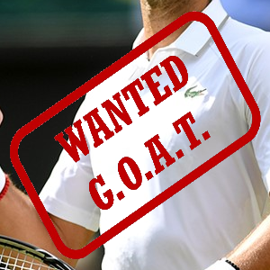
Observe the result. We can see that only the red part has been pasted over the larger image, keeping everything else intact. This final ROI will now be added to the rest of the image in the exact same way as we learnt earlier. We will overlay this final ROI over the original larger image such that the smaller image is now equal to the final ROI.
small_img = final_roiFollowing the steps for overlaying method, we will perform NumPy indexing to achieve the final result.
large_img[y_offset : y_offset + small_img.shape[0], x_offset : x_offset + small_img.shape[1]]= small_img
cv2_imshow(large_img)
Output:

There you go! The two images have been successfully blended without any disturbance from the white background of the overlaying smaller image.
Well, that’s it for the blog. We hope you will continue to read up more about blending and pasting, and tell us which examples you took to practise these concepts. Before you go, let’s refresh the topic we learnt today.
Blending and Pasting of Images Using OpenCV
- Blending is the mixing of two images on top of each other
- Images of same size are easier to blend
- Images of different sizes need the creation of mask and is a slightly more complicated blending process
- Blending for images of varying sizes involves three stages: selecting, masking and overlaying
Summary
So that was our tutorial post on blending and pasting images. It is clear that blending images of varying sizes finds applications in many day-to-day projects especially graphic designing. You can have a lot of fun with these concepts using your own examples. While we told you our tennis favorites today, do share with us who you think is the GOAT in other sports like football or basketball. Leave us a comment, ok? Until next time, ‘Blend It Like Beckham!’.
