Highlights: In this post, we’re going to talk about the most common object tracking algorithms – Mean-Shift and CAMShift (Continuously Adaptive Mean-Shift). First, we are going to describe the theory behind the Mean-Shift algorithm. Then, we’ll explain how to apply this algorithm for object tracking in OpenCV with Python. Finally, we’ll learn how to extend the Mean-Shift algorithm into a CAMShift algorithm. So, let’s begin.

Tutorial Overview:

1. Mean-Shift algorithm – introduction
2. Calculating the Man-Shift
   • The Mean-Shift vector example
   • Understanding the idea of the Mean-Shift algorithm
   • Kernel Density Estimation
3. Mean-Shift algorithm in Python
   • Understanding Object Tracking with Mean-Shift algorithm
4. CAMShift algorithm
5. CAMShift algorithm in Python

1. Mean-Shift algorithm – introduction

First, let’s explain how the Mean-Shift algorithm works. It is a powerful clustering algorithm used in unsupervised learning. Sometimes it is known as a mode-seeking algorithm developed by Fukunaga and Hostetler back in 1975. It is very similar to another popular clustering algorithm called the K-means algorithm. However, unlike K-means it does not make any assumptions. In other words, with Mean-Shift, we do not need to specify the number of clusters in advance because that number will be determined by the algorithm automatically. Therefore, we can say that it is a non-parametric algorithm.

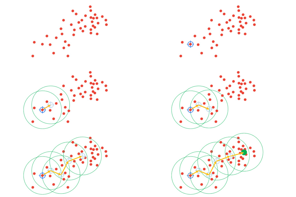
Now, let’s visualize how actually Mean-Shift algorithm works by looking at the following GIF animation.

The goal of the mean-Shift algorithm is to find a region of the highest density. In the example above we can see that Mean-Shift works by grouping data points into clusters. Then, the algorithm converges the cluster centers towards the highest density of data points.

Now, with the KMeans algorithm, we start by randomly selecting cluster centers. On the other hand, with Mean-Shift, we will initially choose a point. Note that here, every feature point can potentially be a cluster center. Next, we will assume a circular region of interest (or kernel) centered around one random point with a radius \(r \).  Once we have our kernel, we are going to calculate the mean of all data points within the circle. Then, the location of the new centroid will be updated. That will give us a vector from a previous location to the mean of the new location. This vector is called the Mean-Shift vector. Once we have a new mean we will continue to shift the kernel iteratively to a higher-density region. We will repeat this procedure while eventually, the Mean-Shift vector is equal to 0. That means that we have converged to a final cluster center and that we have reached the highest density region.

Note, that when we apply the same process to every single point, all points in one cluster should reach this exact same cluster center at the end of the process.

So, let’s summarize how the Mean-Shift algorithm works.

1. We start with the data points assigned to a cluster 
2. The algorithm will compute the centroids.
3. The location of the new centroids will be updated.
4. The process will be iterated and moved to a higher-density region.
5. The process will be finished once the centroids reach a position from where they cannot move further

So, this was a brief introduction to the Mean-Shift algorithm. Now, let’s understand and describe the Mean-Shift method in more detail.

2. Calculating the Mean-Shift

The Mean-Shift vector example

Every shift of data point is defined by a Mean-Shift vector which always points toward the maximum density increase. So, let’s see how we can calculate this vector.

Suppose that we have a starting data point \(y_{0} \) located in the center of an initial cluster. We will calculate the mean of all two-dimensional points in the cluster \(x_{i} \), by summing them up and dividing them by the total number of points. Then, we will subtract the initial estimate \(y_{0} \) from that equation.

$$ M_{h}(\mathbf{y})=\left[\frac{1}{n_{x}} \sum_{i=1}^{n_{x}} \mathbf{x}_{i}\right]-\mathbf{y}_{0} $$

Now, to calculate the Mean-Shift we need to assign a weight \(w_{i} \) to each point in the cluster. That weight depends on the distance from the initial point \(y_{0} \) to a particular point.

$$ M_{h}\left(\mathbf{y}_{0}\right)=\left[\frac{\sum{i=1}^{n_{x}} w_{i}\left(\mathbf{y}_{0}\right) \mathbf{x}_{i}}{\sum_{i=1}^{n_{x}} w_{i}\left(\mathbf{y}_{0}\right)}\right]-\mathbf{y}_{0} $$

Where,

• \(n_{x} \) – number of points in the kernel
• \(y_{0} \) – initial mean location
• \(x_{i} \) – input samples
• \(h \) – radius of a kernel

Understanding the idea of the Mean-Shift algorithm

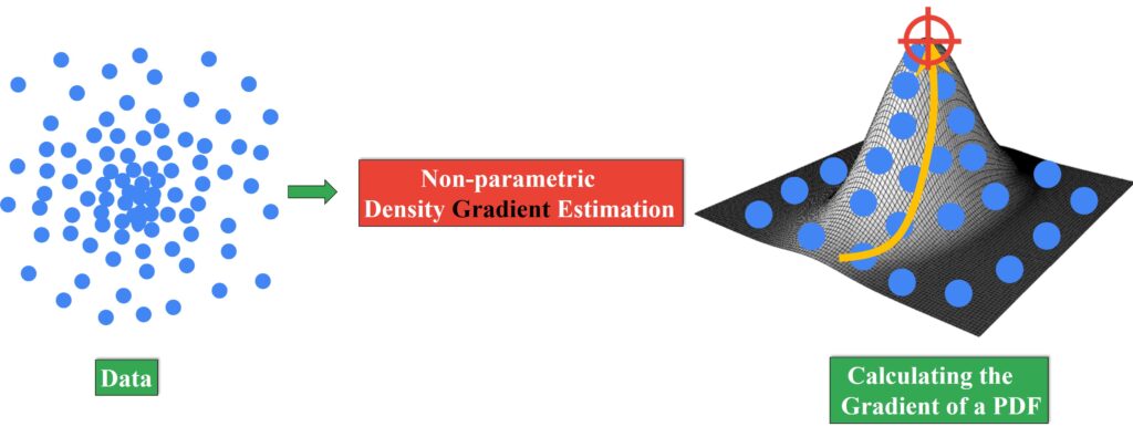
Usually, when we want to analyze the distribution of data points we can use different types of parametric distributions. For example, in Gaussian distribution, once we have samples we can compute the parameters and have a simple description of a density function. The problem with this approach is that often we will not be able to fit the Gaussian distribution to our samples. If that is the case we need to use the non-parametric distribution. To analyze the non-parametric distribution we can use the Mean-Shift algorithm. The idea of the Mean-Shift is to find modes (peak areas) of data points that can be used for shaping a kernel-based estimate of a probability density function.

We can better understand this by looking at the following image.

On the left side, we can see our data points and on the right side, we can see a representation of a probability density function in 3D for this dataset. So, how can we calculate the peak of this probability density distribution? As we have already explained at each kernel we obtain the maximum density in the local neighborhood. Then, we can find the peak by calculating the gradient of this distribution. We will start at the base of the hill and our goal is to reach the point located at top of the hill. One important property that the Mean-Shift vector has is that it is always in the direction of the gradient of the density estimate. So, by calculation of the Gradient, we will move toward the top of the hill. until we reach the maximum density. This algorithm is called the Gradient ascent algorithm.

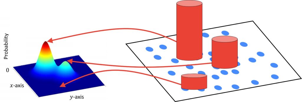
We can create a probability density function by calculating the distance between an initial estimate \(y \), and all other sample points. In that way, all points in the data set will contribute to the probability of \(y \), and that contribution will depend on how close they are to the \(y \). So basically, we are mapping points from the dataset to a histogram where every value will represent a probability of a density for a given point. In other words, a data point density will imply the histogram value.

In the image above we can see an illustration of how we can map data points to a histogram of the probability density function. Another common way to represent the density is to use a height of a bin where height is proportional to the higher density of a point.

Kernel Density Estimation 

In order to represent density distribution in a non-parametric way, we are going to use Kernel Density Estimation. In statistics, Kernel Density Estimation (KDE) is a non-parametric way to estimate the probability density function of a random variable.

Now, let’s see how we can estimate the Probability Density Function in 1D. Let’s say that we have a sample of data points and we want to find an approximation of the PDF from this sample. We can do this in the following way:

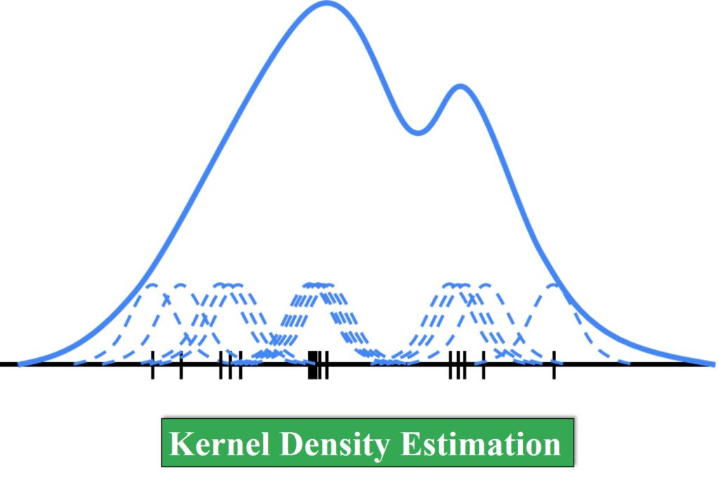
On the left side, you can see our sample points. Now, you can imagine that there is a small bump that represents each of these data points. Our goal is to map all these data points to a histogram of the Probability Density Function that you can see on the right. To do that we can use these small bumps and sum them in order to get an approximation of the PDF.

For the small bumps, we can take a Gaussian function. This Gaussian function will be multiplied by a certain coefficient \(c_{i} \). In that way when we sum these small bumps (Gaussian distributions) and the result should add to the area under this big curve. So. we can write an equation for the PDF in the following way:

$$ p(\mathbf{x})= \sum_{i}c_{i}e ^{-\frac{(x-\mu_{i})^{2}}{2\sigma ^{2}}} $$

Kernel function

Next, we need to define a kernel function. This function can be interpreted as the distance between two points.

$$ K\left(\boldsymbol{x}, \boldsymbol{x}^{\prime}\right) $$

There are different types of kernels like Gaussian, Uniform, or Epanechinkov kernels that we can choose.

• Gaussian, normal or exponential kernel – Assigns weights that depend on the distance between data points.

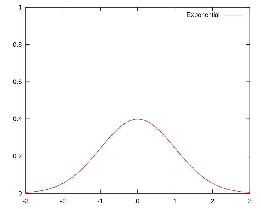
$$ K\left(\boldsymbol{x}, \boldsymbol{x}^{\prime}\right)=c \exp\left(-\frac{1}{2}\left\|\boldsymbol{x}-\boldsymbol{x}^{\prime}\right\|^{2}\right) $$

• Uniform kernel – Assigns always the same weights, regardless of the distance between the points.

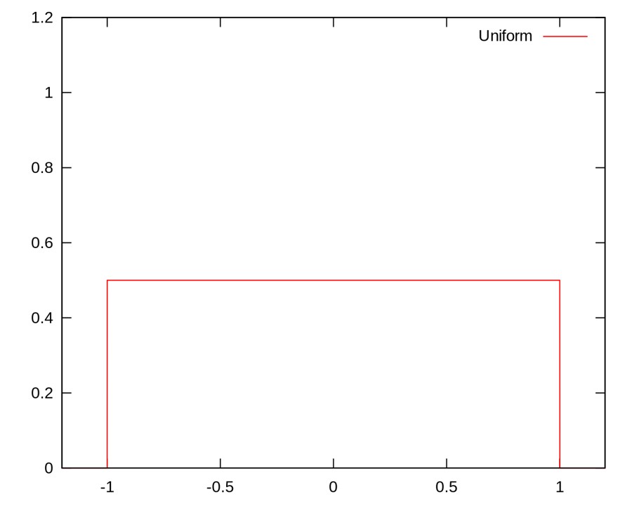
$$ K\left(\boldsymbol{x}, \boldsymbol{x}^{\prime}\right)=\left\{\begin{array}{ll}c & \left\|\boldsymbol{x}-\boldsymbol{x}^{\prime}\right\| \leq 1 \\0 & \text { otherwise } \end{array}\right. $$

• Epanechnikov (parabolic) kernel – is a special kernel that has the lowest (asymptotic) mean square error.

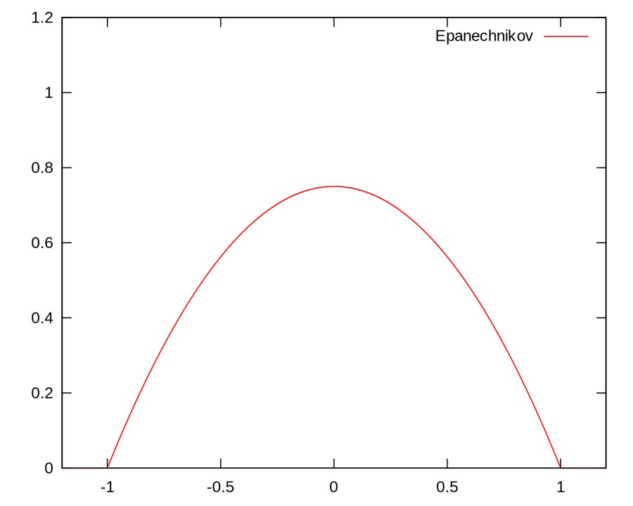
$$ K\left(\boldsymbol{x}, \boldsymbol{x}^{\prime}\right)=\left\{\begin{array}{ll}c\left(1-\left\|\boldsymbol{x}-\boldsymbol{x}^{\prime}\right\|^{2}\right) & \left\|\boldsymbol{x}-\boldsymbol{x}^{\prime}\right\|^{2} \leq 1 \\0 & \text { otherwise }\end{array}\right. $$

These are examples of how we can apply different weights by using different kernel functions. Now, let’s move on.

Connecting KDE, and the Mean-Shift Algorithm

The main idea that we can include is to connect Kernel Density Estimation and the Mean-Shift algorithm.  

So, let’s consider the set of points:

$$ \left\{\boldsymbol{x}_{s}\right\}_{s=1}^{S} \quad \boldsymbol{x}_{s} \in \mathcal{R}^{d} $$

These points lie in a 2D plane. In that case, \(d \) is equal to 2, but also it can be some higher dimension. Next, we sample the mean using the following formula.

$$ m(\boldsymbol{x})=\frac{\sum_{s} K\left(\boldsymbol{x}, \boldsymbol{x}_{s}\right) \boldsymbol{x}_{s}}{\sum_{s} K\left(\boldsymbol{x}, \boldsymbol{x}_{s}\right)} $$

Here, the \(K \) is the sum of the kernels. For example, if we have a Gaussian kernel, we can just plug in the formula for the Gaussian kernel from the previous example. In that case, if we are very close to the center, we will have a high weight, and if we are far away from the center, the impact will be lower. Eventually, the impact will be zero if we are very far away from the center. So, this is the idea of how we can mathematically model this concept. The important point is that we are taking this sum over all data that we have. If we have calculated the current mean \(m(x) \), and we want to get an updated mean, we don’t want to take into account all points in the kernel. Our goal is to give the largest impact to the points closest to the mean, and a small impact to the points far away from the mean.

This is how the formula for the mean shift looks.

$$ m(\boldsymbol{x})-\boldsymbol{x} $$

Here, \(m(x) \) is a sample mean, and \(x \) is an initial point. The idea of the Mean-Shift algorithm is that we need to move from each data point to its mean \(x\leftarrow m(x) \), and iterate until \(x=m(x) \). In other words, we will iterate until the mean stops changing significantly. 

Now, let’s see how the KDE is related to the Mean-shift algorithm.

Radially symmetric kernel

As we have already explained at the beginning of the process we assume a circular kernel centered around one random point. It is important to note here that if the distance between two points and the center of the kernel is the same, they will have the same value. This type of kernel is also called Radially symmetric kernel and it can be expressed in the following way:

$$ K\left(\boldsymbol{x}, \boldsymbol{x}^{\prime}\right)=c \cdot k (\left \| \boldsymbol{x}-\boldsymbol{x}^{\prime} \right \|) ^{2} $$

Relation between KDE and Mean-shift algorithm

Now, we can express our kernel function as the sum of terms of the Radially symmetric kernel:

$$ P(\boldsymbol{x})=\frac{1}{n} c \sum_{n} k(\left \| \boldsymbol{x}-\boldsymbol{x}^{\prime} \right \|) ^{2} $$

This is our kernel density estimate function with radially symmetric kernels. Earlier in the post, we already explained that the Gradient of a PDF is related to the mean shift vector. So, we can say that the Mean-Shift is a ‘step’ in the direction of the gradient of the KDE.

$$ \nabla P(\boldsymbol{x}) \propto m(\boldsymbol{x}) $$

Next, let’s assume that you want to find the maximum of the PDF. To do that, we can calculate a gradient of the kernel function with respect to \(x \). 

$$ \nabla P(\boldsymbol{x})=\frac{1}{n} c \sum_{n} \nabla k\left(\left\|\boldsymbol{x}-\boldsymbol{x}_{n}\right\|^{2}\right) $$

Now, we will calculate a partial derivative or gradient of the kernel itself. 

$$ \nabla P(\boldsymbol{x})=\frac{1}{n} 2 c\sum_{n}\left(\boldsymbol{x}-\boldsymbol{x}_{n}\right) k^{\prime}\left(\left\|\boldsymbol{x}-\boldsymbol{x}_{n}\right\|^{2}\right) $$

Now, let’s change the notation and just replace the kernel derivative within the following expression. 

$$ k^{\prime}(\cdot)=-g(\cdot) $$

When we change the notation everything remains the same, and only \(x \) and \(x_{n} \) change places because here we added minus.

$$ \nabla P(\boldsymbol{x})=\frac{1}{n} 2 c\sum_{n}\left(\boldsymbol{x}_{n}-\boldsymbol{x}\right) g\left(\left\|\boldsymbol{x}-\boldsymbol{x}_{n}\right\|^{2}\right) $$

The next step is to multiply out this equation with \((x_{n} -x) \).

$$ \nabla P(\boldsymbol{x})=\frac{1}{n} 2 c \sum_{n} \boldsymbol{x}_{n}g\left(\left\|\boldsymbol{x}-\boldsymbol{x}_{n}\right\|^{2}\right)-\frac{1}{n} 2 c \sum_{n} \boldsymbol{x} g\left(\left\|\boldsymbol{x}-\boldsymbol{x}_{n}\right\|^{2}\right) $$

Now, this long function can be simplified. We can write it in shorthand notation:

$$ g\left(\left\|\boldsymbol{x}-\boldsymbol{x}_{n}\right\|^{2}\right) =g_{n} $$

$$ \nabla P(\boldsymbol{x})=\frac{1}{n} 2 c \sum_{n} \boldsymbol{x}_{n} g_{n}-\frac{1}{n} 2 c \sum_{n} \boldsymbol{x} g_{n} $$

Now, we can apply one useful trick. We will multiply the first part of the equation by the following term:

$$ \frac{\sum_{n} g_{n}}{\sum_{n} g_{n}} $$

Here, we have the sum of kernels divided by the sum of kernels, which is equal to 1.  So, our equation multiplied by this term will look like this:

$$ \nabla P(\boldsymbol{x})=\frac{1}{n} 2 c \sum_{n} \boldsymbol{x}_{n} g_{n}\left(\frac{\sum_{n} g_{n}}{\sum_{n} g_{n}}\right)-\frac{1}{n} 2 c \sum_{n} \boldsymbol{x} g_{n} $$

$$ \nabla P(\boldsymbol{x})=\frac{1}{n} 2 c \sum_{n} g_{n}\left(\frac{\sum_{n} \boldsymbol{x}_{n} g_{n}}{\sum_{n} g_{n}}-\boldsymbol{x}\right) $$

So, this is the final term. Does this look familiar? Well, yes. We can see that inside the bracket we have our mean shift. 

This proves that the mean shift is a step in the direction of the gradient of the kernel density estimate. If we calculate the mean shift that would correspond to gradient descent with adaptive step size. 

$$ m(\boldsymbol{x})=\left(\frac{\sum_{n} \boldsymbol{x}_{n} g_{n}}{\sum_{n} g_{n}}-\boldsymbol{x}\right)=\frac{\nabla P(\boldsymbol{x})}{\frac{c}{n} \sum_{n} g_{n}} $$

As you can see, we have proven that the Mean Shift is basically the gradient of the non-parametric probability density function. So, calculating the mean and shifting the kernel to the new location until convergence is actually a process of calculating the gradient of the distribution of the points. In this process, we are always moving in the direction of the gradient of the density estimate. In other words, we are climbing to the top of the hill. That is why the goal of the Means-Shift algorithm is to find the peak of the probability density function.

Now, let’s see how we can apply the Means-shift algorithm to images.

Applying the Mean-Shift algorithm on images

Object tracking with a Mean-Shift algorithm can be divided into three stages:

• Target the object – In the first frame, we choose the initial location of the object that we want to track. Then we represent the target model with a color histogram. When the object moves, this movement will be reflected in the histogram.
• Finding the new location – In the next frame, the Mean-Shift algorithm moves the window to the new location with maximum pixel density. Now, we use the current histogram to search for the best target match candidate by maximizing the similarity function.
• Updating the location – We update the histogram and the location of the target object.

To better understand object tracking with the mean-Shift algorithm let’s have a look at the following image.

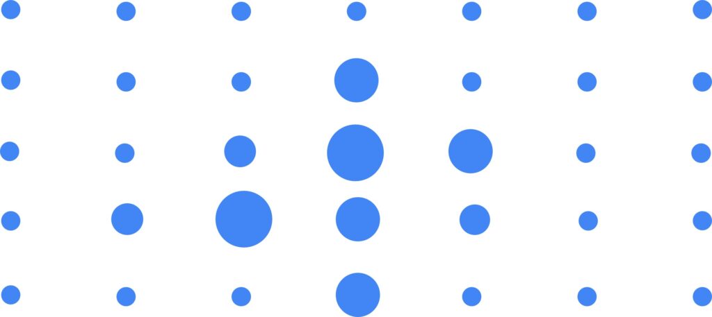
Every point on the image above represents one pixel. Notice that each pixel is a point with a certain weight. We need to assign a weight to a pixel because otherwise, we wouldn’t be able to apply the Mean-Shift algorithm. Now, the crucial thing here is to figure out how a certain pixel can have weight. 

Let’s assume that we want to track an object in a video. In the first frame, we choose the initial location of the object that we want to track. We will define an area around our target object. Once our target object moves we want to find the best candidate location for the object in the second frame. 

The problem that we need to solve is how to model the target and candidate regions. We can represent the target model with a normalized color histogram which is weighted by the distance. 

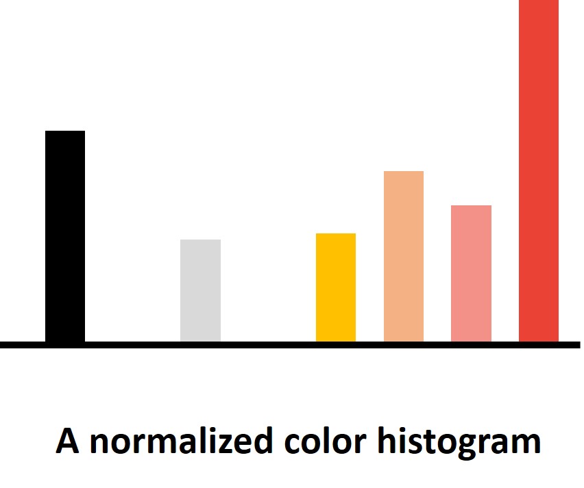
Here, if a pixel is closer to the center it will provide more weight, and pixels that are further to the center will contribute less to this histogram.

Describing the Target model

One option to describe the target model is to use an M-dimensional target descriptor centered at the target center. 

$$ \boldsymbol{q}=\left\{q_{1}, \ldots, q_{M}\right\} $$

To calculate the M-dimensional target descriptor we can use the following formula:

$$ q_{m}=C \sum_{n} k\left(\left\|\boldsymbol{x}_{n}\right\|^{2}\right) \delta\left[b\left(\boldsymbol{x}_{n}\right)-m\right] $$

Here, \(C \) is the Normalization factor, then we have the function of inverse distance(weight). The last part of the formula is called the Kronecker delta function. It tells us that if we are far away from the center of this ladybug. So, if the pixel is further from the center, the lower this value will be. On the other hand, if we are close to the center, that pixel will have a higher impact.

So, we first pick a center, and then we need to scan all the pixels around this target. For example, let’s say that we want to calculate the M-dimensional target descriptor for all dark pixels. To do that we can split the colors into bins. Then if the pixel is not dark, this value will be zero. On the other hand, if it is a dark pixel, our result will be 1. We will count the distance from the center, and this distance will affect how much we will increase this black bin in the color histogram.

After we have described our target model, we move on to the next step of the Mean-Shift method which is about describing the object candidate model.

Describing the candidate model

In the image below we can see that the yellow circle is the candidate for the target. Imagine the ladybug from the previous example has moved and it now has a new center and we need to find this new center of the candidate region \(y\). To do that we will calculate the M-dimensional histogram that will represent this yellow circle. We will calculate this histogram in the same way as we did for the target model. We can start from the center \(y \) and scan all pixels that are in the yellow circle. The pixels closer to the center will provide more impact on the histogram values, and pixels that are further from the center will contribute less to these histogram values.

Then using a Mean-shift we will move the center until we find the best match.

$$ \boldsymbol{p}(\boldsymbol{y})=\left\{p_{1}(\boldsymbol{y}),\ldots, p_{M}(\boldsymbol{y})\right\} $$

The similarity between the Target and Candidate Models 

After we model our target and candidate region, we need to determine the degree of similarity between them. To do that, we just need to calculate the difference between two histograms. For that, we will use two functions. First is the distance function which will help us to calculate the distance \(d(y) \) between the center of the candidate region \(y \) and the target descriptor \(q \). 

$$ d(\boldsymbol{y})=\sqrt{1-\rho[\boldsymbol{p}(\boldsymbol{y}), \boldsymbol{q}]} $$

Also, we will use the Bhattacharya coefficient, which can be expressed in the following way:

$$ \rho(y) \equiv \rho[\boldsymbol{p}(\boldsymbol{y}), \boldsymbol{q}]=\sum_{m} \sqrt{p_{m}(\boldsymbol{y}) q_{u}} $$

The Bhattacharyya coefficient is an approximate measurement of the amount of overlap between two statistical samples. In our case, these samples are two histograms. Usually, this coefficient ranges between 0 and 1. The larger the value of this coefficient, the more similar the object and the candidate models.

Now, we will calculate the cosine distance between two unit vectors using the following equation:

$$ \rho(\boldsymbol{y})=\cos \theta \boldsymbol{y}=\frac{\boldsymbol{p}(\boldsymbol{y})^{\top} \boldsymbol{q}}{\|\boldsymbol{p}\|\|\boldsymbol{q}\|}=\sum_{m} \sqrt{p_{m}(\boldsymbol{y}) q_{m}} $$

Now, let’s see how we can maximize the Bhattacharya coefficient and minimize the distance function in order to make the two models more similar.

Maximizing the similarity between the target and candidate model

This is just mathematical proof of how you can actually minimize this distance function or maximize the similarity between our target histogram and candidate histogram.

We can express this process mathematically in the following way:

$$ \min _{\boldsymbol{y}} d(\boldsymbol{y}) \quad \text { same as } \quad \max _{\boldsymbol{y}} \rho[\boldsymbol{p}(\boldsymbol{y}), \boldsymbol{q}] $$

First, we will assume a good initial guess:

$$ \rho\left[\boldsymbol{p}\left(\boldsymbol{y}_{0}+\boldsymbol{y}\right), \boldsymbol{q}\right] $$

Next, we will linearize around the center of the object from the initial frame \(y_{0} \) and then look for the best matching object center in the current frame, represented by \(y_{1} \). We will use a Taylor series expansion to start in the neighborhood such that the distance between the starting point \(y_{0} \) and the target point \(y_{1} \) doesn’t become too large. In case it becomes too large as in the case of fast object movement, the Mean-Shift algorithm tracking effect is not ideal.

$$ \rho[\boldsymbol{p}(\boldsymbol{y}), \boldsymbol{q}] \approx \frac{1}{2} \sum_{m} \sqrt{p_{m}\left(\boldsymbol{y}_{0}\right) q_{m}}+\frac{1}{2} \sum_{m} p_{m}(\boldsymbol{y}) \sqrt{\frac{q_{m}}{p_{m}\left(\boldsymbol{y}_{0}\right)}} $$

$$ p_{m}=C_{h} \sum_{n} k\left(\left\|\frac{y-x_{n}}{h}\right\|^{2}\right) \delta\left[b\left(\boldsymbol{x}_{n}\right)-m\right] $$

Now, let’s expand on this term:

$$ \rho[p(\boldsymbol{y}), \boldsymbol{q}] \approx \frac{1}{2} \sum_{m} \sqrt{p_{m}\left(\boldsymbol{y}_{0}\right) q_{m}}+\frac{1}{2} \sum_{m}\left\{C_{h} \sum_{n} k\left(\left\|\frac{\boldsymbol{y}-\boldsymbol{x}_{n}}{h}\right\|^{2}\right) \delta\left[b\left(\boldsymbol{x}_{n}\right)-m\right]\right\} \sqrt{\frac{q_{m}}{p_{m}\left(\boldsymbol{y}_{0}\right)}} $$

After moving terms around we will get the following equation:

$$ \rho[\boldsymbol{p}(\boldsymbol{y}), \boldsymbol{q}] \approx \frac{1}{2} \sum_{m} \sqrt{p_{m}\left(\boldsymbol{y}_{0}\right) q_{m}}+\frac{C_{h}}{2} \sum_{n} w_{n} k\left(\left\|\frac{\boldsymbol{y}-\boldsymbol{x}_{n}}{h}\right\|^{2}\right) $$

where,

$$ w_{n}=\sum_{m} \sqrt{\frac{q_{m}}{p_{m}\left(\boldsymbol{y}_{0}\right)}} \delta\left[b\left(\boldsymbol{x}_{n}\right)-m\right] $$

Here we have two terms. The first one is not dependent on \(y \), and this second one is actually the weighted kernel density estimate. So, we only need to maximize the second term. To do that we will use the Mean-Shift algorithm.

$$ \frac{C_{h}}{2} \sum_{n} w_{n} k\left(\left\|\frac{\boldsymbol{y}-\boldsymbol{x}_{n}}{h}\right\|^{2}\right) $$

$$ y_{1}=\frac{\sum_{n} \boldsymbol{x}_{n} w_{n} g\left(\left\|\frac{\boldsymbol{y}_{0}-\boldsymbol{x}_{n}}{h}\right\|^{2}\right)}{\sum_{n} w_{n} g\left(\left\|\frac{\boldsymbol{y}_{0}-\boldsymbol{x}_{n}}{h}\right\|^{2}\right)} $$

So, let’s summarize the Mean-Shift tracking procedure:

1. Initialize location \(\boldsymbol{y}_{0}\)
   • Compute \(q \)
   • Compute \(\boldsymbol{p}\left(\boldsymbol{y}_{0}\right) \)
2. Derive weights \(\boldsymbol{w}_{n} \)
3. Shift to new candidate location (mean shift) \(\boldsymbol{y}_{1} \)
4. Compute \(\boldsymbol{p}\left(\boldsymbol{y}_{1}\right) \)
5. If \(\left\|\boldsymbol{y}_{0}-\boldsymbol{y}_{1}\right\|<\epsilon \) return
   • Otherwise \(\boldsymbol{y}_{0} \leftarrow \boldsymbol{y}_{1} \) and go back to \(2 \)

2. Mean-Shift algorithm in Python

Understanding Object Tracking with Mean-Shift algorithm

This process of object tracking with the Mean-Shift algorithm is illustrated in the image below.

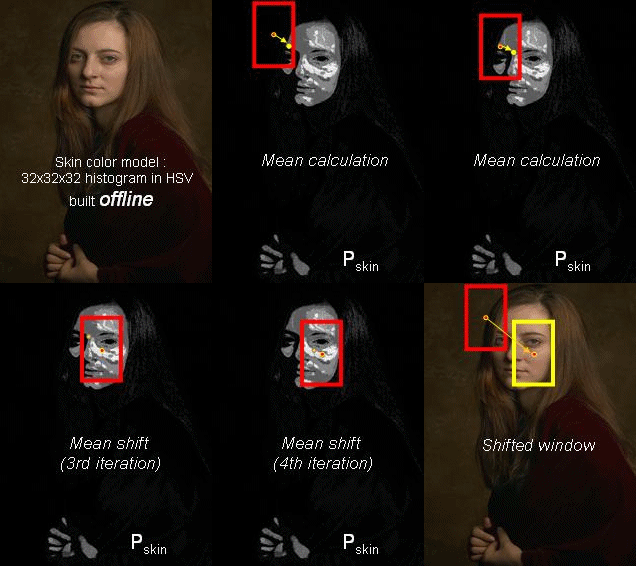
Now, let’s write a code for object tracking with the Mean-Shift algorithm. First, let’s import the necessary libraries.

# Necessary imports
import numpy as np
import cv2
from google.colab.patches import cv2_imshow
import matplotlib.pyplot as plt

With the following command, we will download the video sequence directly to our Python script. Then, we will load the video, define the fourcc codec, and create a VideoWriter object.

!wget https://raw.githubusercontent.com/maticvl/dataHacker/master/DATA/usain_bolt.mp4 -O "usain_bolt.mp4"

# Creating a VidoCapture and VideoWriter object
cap=cv2.VideoCapture("usain_bolt.mp4")
ret, frame = cap.read()
fourcc = cv2.VideoWriter_fourcc('M','J','P','G')
out = cv2.VideoWriter('output.avi', fourcc, 29, (1280, 720))

Now, we will manually set up our initial location of a tracking window. Our intention is to detect one object in the first frame of the video and draw a rectangle around it. Then we need to extract the location and dimensions of an ROI (region of interest). The idea is to treat pixels inside the ROI are the pixels that we need to track. Afterward, we will apply the Mean-Shift algorithm to that ROI. So, let’s see how we can do that.

body_rects = (620, 310, 40, 40)
(x, y, w, h) = body_rects
track_window = (x, y, w, h)

The next step is to create our region of interest with the same dimensions as our tracking window. We can do that with the following code. 

roi = frame[y:y+h, x:x+w]

Next, we’re going to apply HSV (hue, saturation, value). color mapping using the function cv2Color(). HSV is an alternative representation of RGB images that is closer to the way how humans perceive color. It has three components: hue, saturation, and value. This color space describes colors (hue or tint) in terms of their shade (saturation or amount of gray) and their brightness value. As parameters, we will pass ROI and convert it from BGR to HSV. Then, we are going to find the histogram to back project the target on each frame in order to calculate the Mean-Shift. For that, we will use the function cv2.calcHlist() which calculates the histogram of a set of arrays. Then, we are going to normalize the histogram array values given a minimum of zero and a maximum of 255. We can do this with the function cv2.normalize(). 

hsv_roi =  cv2.cvtColor(roi, cv2.COLOR_BGR2HSV)
roi_hist = cv2.calcHist([hsv_roi],[0], None,[180],[0,180])
cv2.normalize(roi_hist,roi_hist,0,255,cv2.NORM_MINMAX)

plt.plot(roi_hist)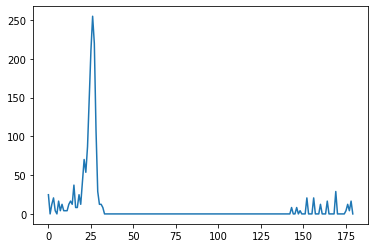

Now, we need to set up the iteration termination criteria. When this criterion is satisfied, the algorithm iteration stops. For that, we will pass two flags. The first is cv2.TERM_CRITERIA_EPS which stops the algorithm iteration if the specified accuracy, epsilon, is reached. The second flag is cv2.TERM_CRITERIA_COUNT which is the maximum number of iterations or elements to compute. So, we are going to go for either 10 iterations or at least one epsilon. Therefore, we will just pass 10, and 1. 

term_crit = ( cv2.TERM_CRITERIA_EPS | cv2.TERM_CRITERIA_COUNT, 10, 1 )

The next step is to create the while loop in order to capture a couple more frames, from the video.

while cap.isOpened():
    ret, frame = cap.read()
    if ret == True:
      hsv = cv2.cvtColor(frame, cv2.COLOR_BGR2HSV)
      dst = cv2.calcBackProject([hsv],[0],roi_hist,[0,180],1)

Inside the loop, we will first grab the first frame and convert it to HSV. Once we have that, we need to calculate the back projection based on the roi_hist that we created earlier. To do that we will use the function cv2.calcBackProject(). This function is used for image segmentation and for detecting objects of interest in an image. It creates an image of the same size as the input image, where each pixel corresponds to the probability of that pixel belonging to the object. As parameters for this function, we will pass HSV that we just got along channel zero, and then we’re going to pass in roi_ hist from 0  to 180.  In the following image, we can see what the first frame from our video looks like after backpropagation.

cv2_imshow(dst)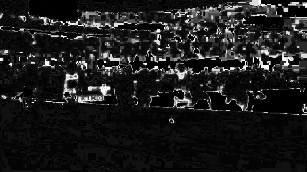

Now, it is time to apply the function cv2.meanShift(). Here we will pass three parameters. First is the back projection that we just calculated. The second parameter is the previous tracking window, and the third parameter is the termination criteria.

# apply Mean-Shift  to get the new location
      ret, track_window = cv2.meanShift(dst, track_window, term_crit)

Then we’re going to draw a new rectangle on the image based on where this new tracking window has been updated. After that, we can break the loop and finally release our output.

#Draw updated rectangle
      x,y,w,h = track_window
      img2 = cv2.rectangle(frame, (x,y), (x+w,y+h), (0,255,0),2)
      out.write(frame)
    else:
      break

out.release()
cap.release()

Output:

As you can see the Mean-Shift algorithm is capable of successfully tracking the greatest sprinter of all time Usain Bolt during one of his famous 100 meters races. However, if we take a closer look at our results we can see that there is a problem. Our window always has the same size whether the object is far away or close to the camera. To fix this problem we need to adapt the window size to the size and rotation of the target. The solution is called the CAMShift algorithm.

3. CAMShift algorithm

The CAMShift algorithm (Continuously Adaptive Mean-Shift) is the first time published in 1998 by Gary Bradsky in his paper “Computer Vision Face Tracking for Use in a Perceptual User Interface” [2]. It is just an extension of the Mean-Shift algorithm that allows us to resize our target window. This algorithm first applies Mean-Shift. Once Mean-Shift finds the mode, it updates the size of the window and also calculates the Roll angle determined by fitting an ellipse to the mode. Then, it applies the Mean-Shift with a new scaled search window and previous window location. The process continues until the required accuracy is met.

4. CAMShift algorithm in Python

The code for the CAMShift algorithm is almost identical to the code for the Mean Shift. The only difference is that the CAMShift algorithm returns a rotated rectangle. Therefore, we will change the way we draw the tracking window because we want it to resize based on the position of the object. 

# Creating a VidoCapture and VideoWriter object
cap=cv2.VideoCapture("usain_bolt.mp4")
ret, frame = cap.read()
fourcc = cv2.VideoWriter_fourcc('M','J','P','G')
out = cv2.VideoWriter('output.avi', fourcc, 25, (1280, 720))

body_rects = (500, 300, 30, 60)
(x, y, w, h) = body_rects
track_window = (x, y, w, h)
roi = frame[y:y+h, x:x+w]

hsv_roi =  cv2.cvtColor(roi, cv2.COLOR_BGR2HSV)
roi_hist = cv2.calcHist([hsv_roi],[0], None,[180],[0,180])
cv2.normalize(roi_hist,roi_hist,0,255,cv2.NORM_MINMAX)
# Setup the termination criteria, either 10 iteration or move by atleast 1 pt
term_crit = ( cv2.TERM_CRITERIA_EPS | cv2.TERM_CRITERIA_COUNT, 10, 1 )

while cap.isOpened():
    ret, frame = cap.read()
    if ret == True:
      hsv = cv2.cvtColor(frame, cv2.COLOR_BGR2HSV)
      dst = cv2.calcBackProject([hsv],[0],roi_hist,[0,180],1)
      
      # apply CAMShift to get the new location
      ret, track_window = cv2.CamShift(dst, track_window, term_crit)

So, after we write the code that is identical to the code we wrote for the Mean-Shift algorithm, we will apply the function cv2.camShift() and pass in the same parameters from the cv2.meanShift() function. Then we will apply the function cv2.boxPoints() which returns the four points of a rotated rectangle. As a parameter for this function, we will pass the returned object from the cv2.camShift() function. Next, we need to convert all points into integers because the function by default returns floating points. And finally, instead of drawing the rectangle, we’re going to draw some polynomial lines. 

#Draw it on image
      pts = cv2.boxPoints(ret)
      pts = np.int0(pts)
      img2 = cv2.polylines(frame,[pts],True, 255,2)
      out.write(frame)
    else:
      break

out.release()
cap.release()

Output:

Now, we can observe our results. This time we tracked one of Bolt’s biggest rivals, Justin Gatlin. As you can see the rectangle will get bigger or smaller depending on the size of the tracking object.  Also, the window will rotate in order to adapt to the position of the object. However, we can also see that this algorithm is not perfect. It is really sensitive to lighting changes. In this particular example, the problem occurs when Gatlin gets closer to the sprinter with the identical red outfit Tyson Gay. For a few seconds, the size of the target window updated and the algorithm started to trace both spriters. Then, when the distance between the two sprinters got longer the algorithm continues to track Gatlin until the end of the video sequence.

Summary

So, that is it for this post. We learned how to track objects with Mean-Shift and CAMShift algorithms. We explained the basic theory behind these algorithms and then we show how to use them in Python. See you soon.

References:

[1] Fukunaga, Keinosuke, and Larry Hostetler. “The estimation of the gradient of a density function, with applications in pattern recognition.” IEEE Transactions on information theory 21.1 (1975).

[2] Bradski, Gary R. “Computer vision face tracking for use in a perceptual user interface.” (1998).

[3] OpenCV: Meanshift and Camshift. (n.d.). https://docs.opencv.org/3.4/d7/d00/tutorial_meanshift.html