Highlight: In this post we will talk about eigenvalues and eigenvectors. This concept proved to be quite puzzling to comprehend for many machine learning and linear algebra practitioners. However, with a very good and solid introduction that we provided in our previous posts we will be able to explain eigenvalues and eigenvectors and enable very good visual interpretation and intuition of these topics. We give some Python recipes as well.

Tutorial Overview:

1. Intuition about eigenvectors
2. Definition of eigenvectors and eigenvalues
3. Example of eigenvector and eigenvalue calculation

1. Intuition about eigenvectors

This post we will start with the following well-known \(\left ( x,y \right ) \) coordinate system.

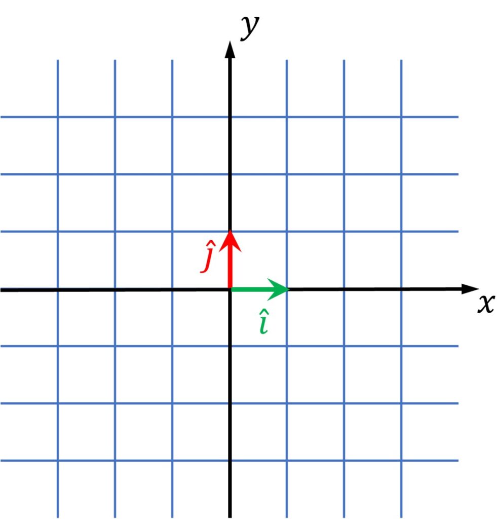
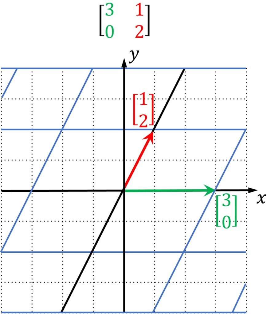
We imagine that we linearly transform this system. We obtain the following transformation where actually our original system is transformed and our \(\hat{i} \) vector is mapped into \(\begin{bmatrix}3\\0\end{bmatrix} \) vector and our \(\hat{j} \) vector is mapped into \(\begin{bmatrix}1\\2\end{bmatrix} \) vector.

Now, in this space we will have some arbitrary vector and this vector is shown in the following image.

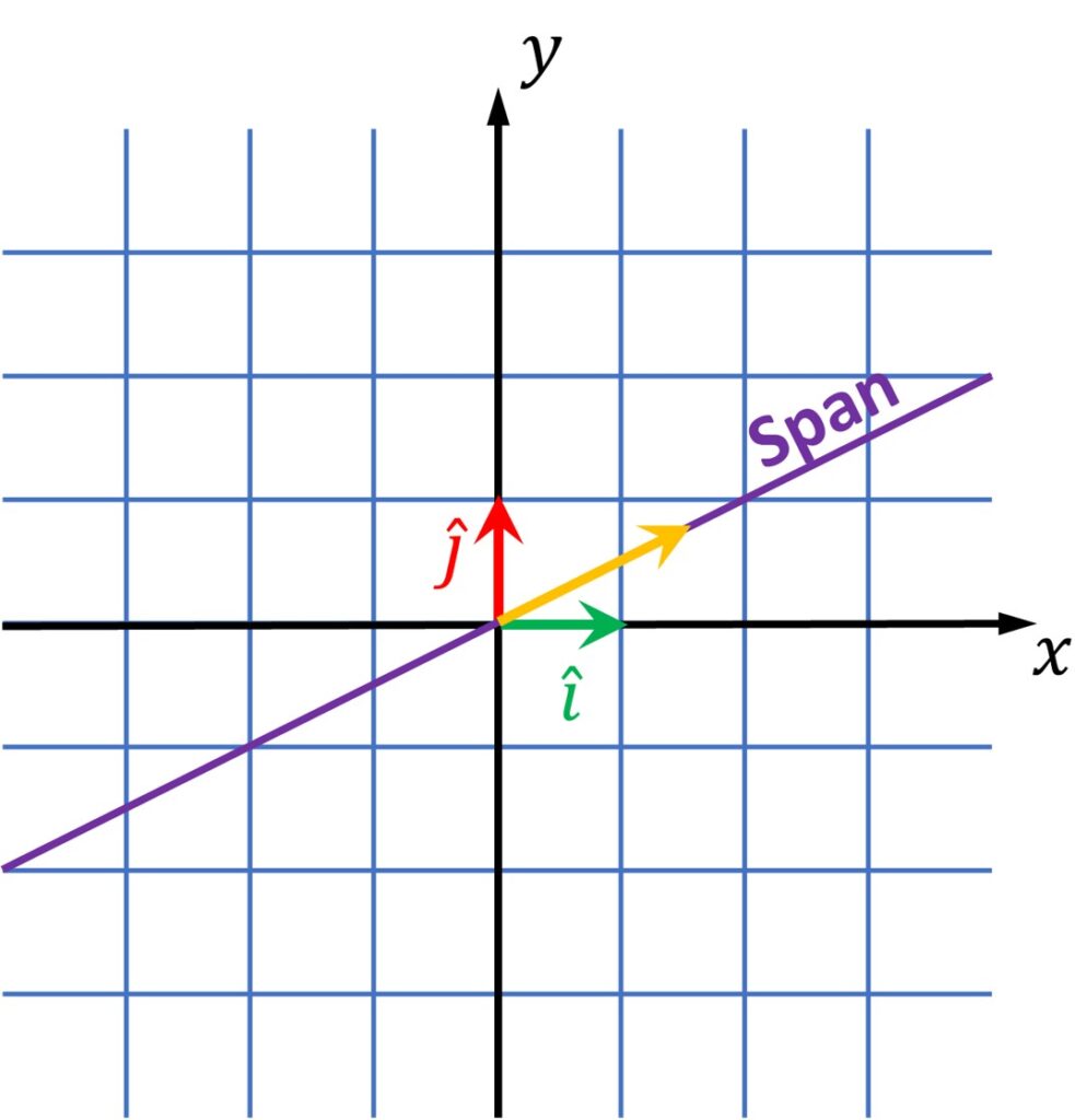
Once we apply a linear transformation to this vector as shown in image below, we see that this vector moved from its original line. It has been knocked off from it . 🙂

However, there will be some particular vectors that will be linearly transformed, and they will remain on their own span. Just too good to be true ?

Sinatra rocks. We know. Ok. But, let’s continue.

The previous idea means that vector will remain on its span line that goes through the origin. Only the vector intensity and/or direction can be changed. We say that this vector is just multiplied by scalar that can stretch this vector, shorten this vector or reverse its direction. Such vectors are called eigenvectors.

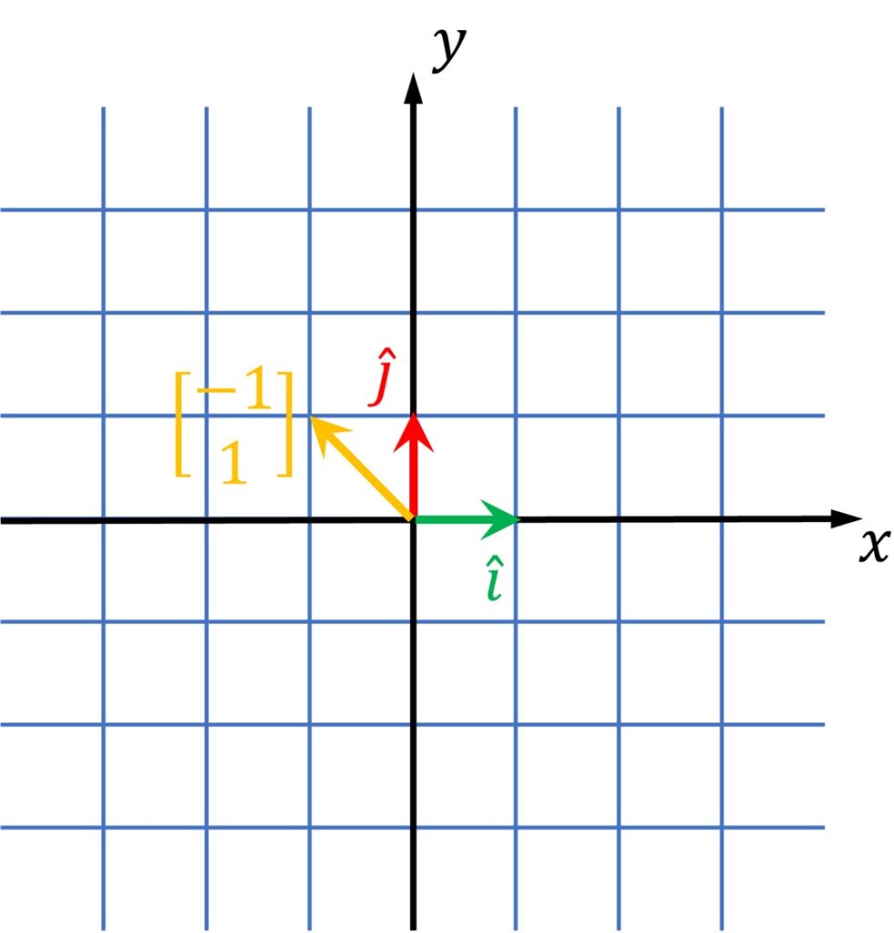
For this particular transformation defined with the matrix \(\begin{bmatrix}3 & 1\\0 & 2\end{bmatrix} \) we will have one particular vector and it’s coordinates are \(\begin{bmatrix}-1\\1\end{bmatrix} \).

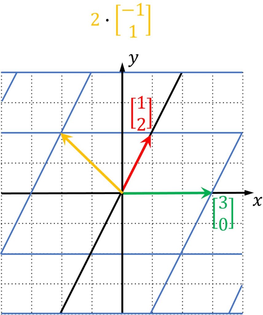
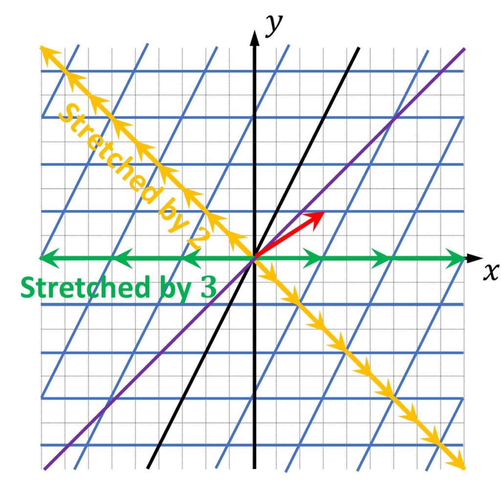
Once we linearly transform this vector, it will be changed by a scalar \(2 \). This means that it will be stretched \(2 \) times. Moreover, a vector \(\begin{bmatrix}1\\-1\end{bmatrix} \) will also be stretched two times with this linear transformation.

In addition, any vector that lies on this line will be stretched by a factor of \(2 \).

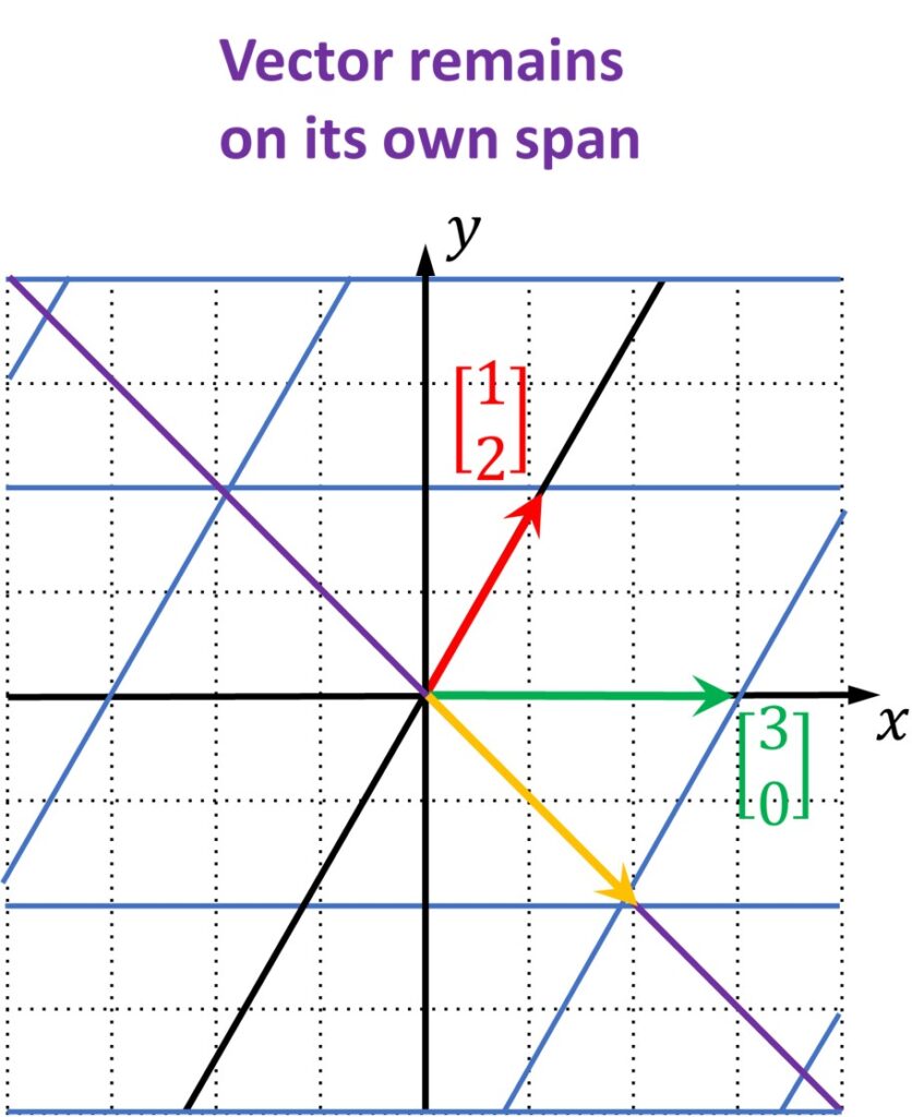
Moreover, in this example, our basis \(\hat{i} \) vector is transformed in such a way that \(\hat{i} \) remains on the \(x\)-axis. This means that any other vector that lies on the \(x\)-axis will remain on this line.

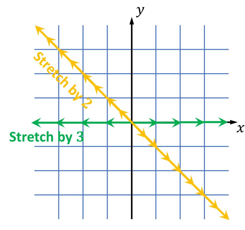
So, this linear transformation matrix has two vectors, that define two lines, and any vector on these lines will remain there after a linear transformation. It is depicted in the image below with yellow and green vectors. In addition, the vectors on the yellow line will be stretched by a scalar 2, whereas the vectors on the green line will be stretched by a scalar 3. These values correspond to the specific eigenvectors and we call them eigenvalues.

On the other hand, once again, we will have all other vectors that actually will not remain on its original line. They will be knocked off from their original line and this is shown in the following image.

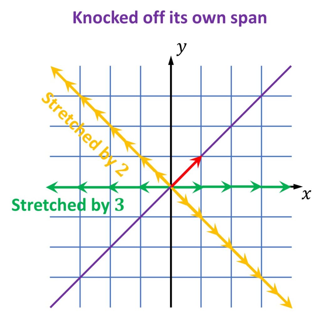
So, once we transform it, we see that this vector (red arrow) will completely go off this line. On the other hand, two vectors, eigenvectors, remain on the same line for this particular transformation.

Where do we use eigenvectors?

One interesting property of eigenvectors can be observed when we apply a rotation transformation on a certain coordinate system. The rotations can be defined along \(x, y, or z \) – axis. However, the axis of rotation can also be arbitrary and unknown. Then, this rotation will be defined by a \(3\times 3 \) matrix for a 3-D space. However, if we manage to find eigenvectors for this rotation matrix, it will define the axis along which this rotation is done. So, this is just one of many applications of eigenvectors.

2. Definition of eigenvectors and eigenvalues

We’ve seen so far how visually eigenvectors can be interpreted and what are eigenvalues. However, we can define it in a more formal way with the following equation:

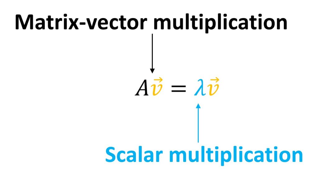
Here, we have the matrix-vector multiplication \(A\cdot \vec{v} \) and that equals vector \(\vec{v} \) multiplied by a scalar. So, we say that the result of \(A\cdot \vec{v} \) will be a vector and it equals the scaled vector \(\vec{v} \). This can be stated as:

For a certain matrix \(A \) we can find a vector \(\vec{v} \) that, when multiplied with the matrix \(A \) will remain on the same line.

The only thing that can change is its intensity and potentially its direction. Commonly, we have a known matrix \(A \). Then, we need to solve this equations for \(\lambda \) and \(\vec{v} \). Those are values that we are looking for.

To solve this equation, we perform the following trick. On the right hand side, we include a matrix vector multiplication and instead to multiply it with a simple scalar we can add the identity matrix. It has ones along the main diagonal. Then, we can extract \(\lambda \) and we will obtain the modified equation \(\lambda\cdot I \) where \(I \) is identity matrix times \(\vec{v} \).

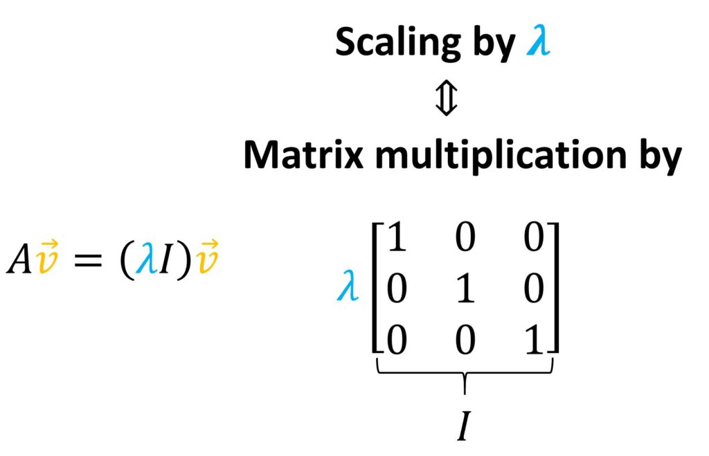
So, if we a little bit modify this equation, we get:

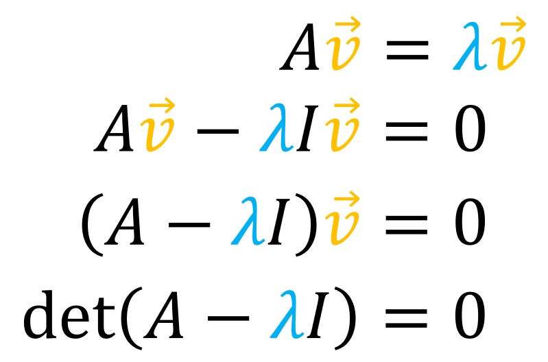
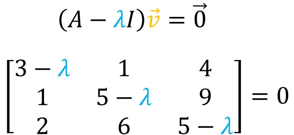
Then, we will have a simple matrix-vector multiplication that should equal a zero vector. Now, our matrix is changed and it is changed with the scalar \(\lambda \). For instance, for this \(3\times 3 \) example we now have our main diagonal \(3-\lambda \), \(5-\lambda \) and once again \(5-\lambda \) 

If we connect this equation with a determinant, we will notice that any vector \(\vec{v} \) multiplied by matrix (whose determinant is not equal to zero), will give us another arbitrary vector.

However, when we have a matrix that multiplies \(\vec{v} \) and we get a zero vector, that can happen only for those values \(\lambda \)s where our determinant of the matrix \(\left ( A-\lambda I \right )= 0 \). Such transformation for those \(\lambda \) will squish the plane into a single line.

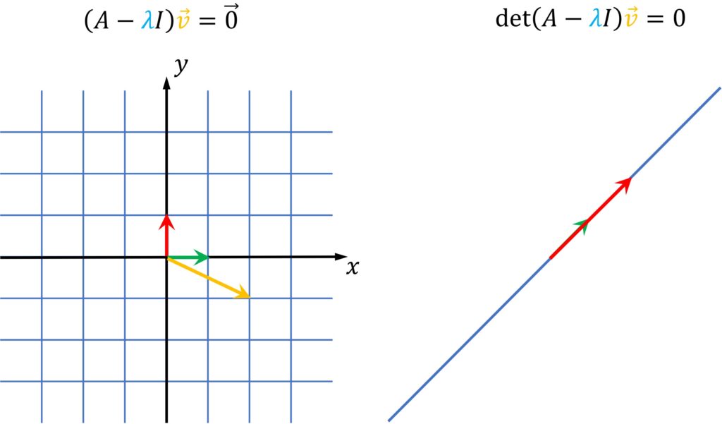
Here is a nice illustration of the parameter \(\lambda \). First, we define a matrix of the linear transformation. So, our goal here will be to change \(\lambda \) and that for different \(\lambda \) we observe the mapping of a coordinate system with this linear transformation.

For instance, let’s say that we start from \(0 \) and we start increasing \(\lambda \)). We can see how the mapping behaves.

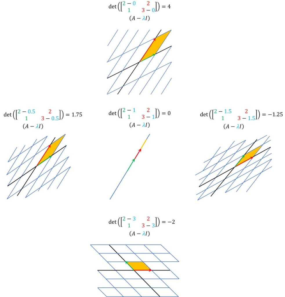
We see that a determinant is getting smaller and smaller. Recall that this is the area of a unit square! At one point it will become zero and exactly at this moment where the determinant is zero, we will obtain a line!

That is, a linear transformation will squash a plane into a line. And this is one of our solutions. And then, if we continue increasing \(\lambda \) we will actually get the negative values of the determinant. So, this can be one way to intuitively try to solve this equation by experimenting with different values of \(\lambda \) and connecting this with how the transformed plane is actually behaving.

3. Example of eigenvector and eigenvalue calculation

Now, let’s work out, our previous example by hand as shown in the image below.

So, if you note that the determinant needs to be zero, we have actually a \(3-\lambda \) and \(2-\lambda \) on the main diagonal. And we know how to solve this. This determinant will be the quadratic equation that we need to solve for different \(\lambda \). And this already implies that most likely we will have not one but two eigenvalues \(\lambda \) because that’s common for quadratic equations. Of course, different scenarios can happen, but as we said the most common is to have two solutions.

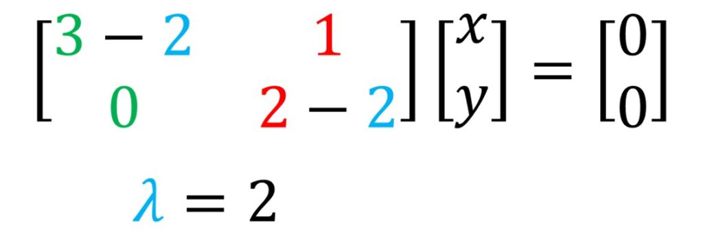
This equation is very easy to solve. it can be solved for \(\lambda = 2 \) or \(\lambda = 3 \) and these values can be actually our eigenvalues.

So, for this \(\lambda \) what we now need to do is to go back to our equation and actually figure out what our vector \(\vec{v} \) actually is. We can replace \(\vec{v} \) as \(x \) and \(y \) and from here and we just need to calculate for what values this is satisfied.

import numpy as np
import matplotlib.pyplot as plt

A = np.array ( [ [3,1] , [0,2] ]  ) 
print(A)

eig_val, eig_vec  =  np.linalg.eig (A)

print("Eigenvalues: ", eig_val)
print("Eigenvectors are columns in the matrix:\n",eig_vec)

Eigenvalues:  [3. 2.]
Eigenvectors are columns in the matrix:
 [[ 1.         -0.70710678]
 [ 0.          0.70710678]]

plt.quiver( [0,0] , [0,0], eig_vec[0,:], eig_vec[1,:], angles = 'xy', scale_units = 'xy', scale = 1  )
plt.xlim(-2, 2)
plt.ylim(-2, 2)
plt.grid('on')
plt.show()
plt.savefig("eigenvectors.png", dpi = 800)

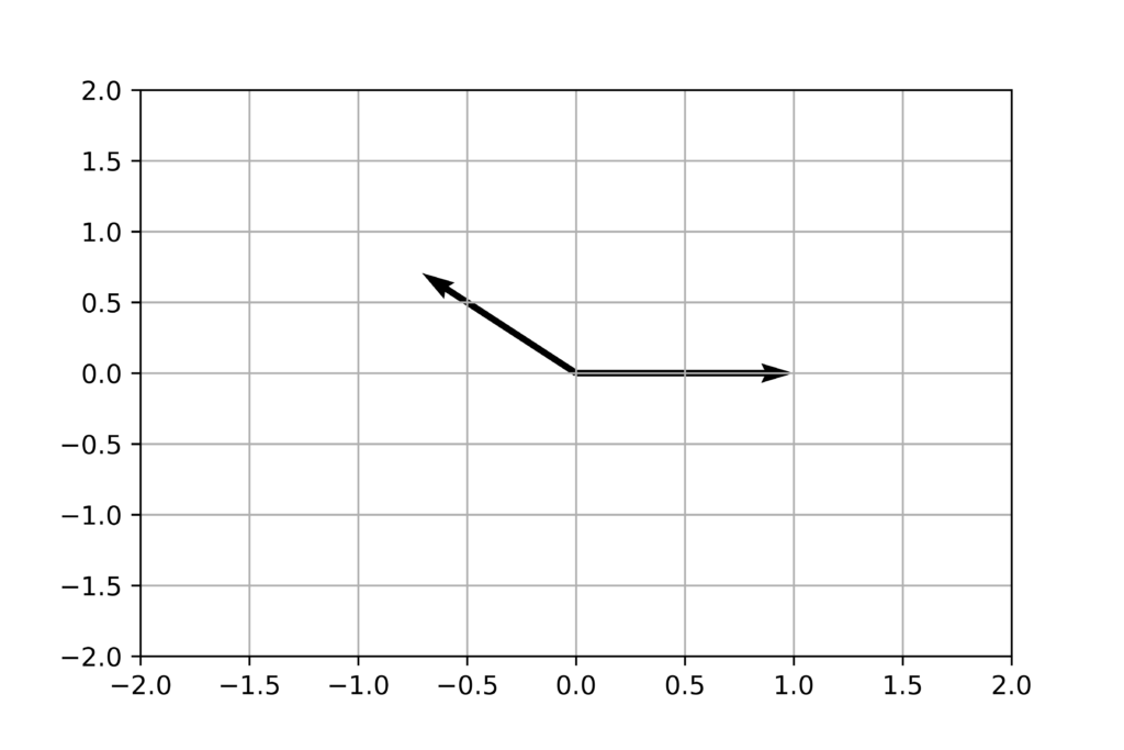
To dive a bit deeper, we can ask ourselves whether eigenvalues always exist?

A rotation matrix. For example, the following matrix is a linear transformation, but what it actually does, it performs rotations. So, if it rotates to the plane for some angle, and in this case \(90^{\circ} \) rotation, we cannot have any vector preserved on the line where it originated from. To confirm this numerically, this will be our determinant for the following rotation matrix. Then we can try to solve this for \(\lambda \) and we will obtain that \(\lambda ^{2}+1= 0 \) . Here, our eigenvalues are complex numbers 🙂

A shear transformation. Another interesting operation can be shear. In this case you can see that the \(x \) – axis or \(\hat{i} \) vector remains the same where the \(\hat{j} \) vector is stretched and inclined. And if you would like to calculate the eigenvectors, we will follow the same principle. So, from this matrix we will subtract \(\lambda \) values and our final equation will be:

So, only one eigenvalue exists and that means that the only eigenvector is actually along the \(x \) – axis.

Eigenvectors and basis change. In addition, one interesting thing to mention is that we learned so far that we can transform our original coordinate system. And it’s quite interesting if we transform it in such a way so that actually eigenvectors of a matrix (we will assume that there are two eigenvectors in this case) we use as a new basis. Then, it’s interesting how actually our new world that’s composed of eigenvectors will behave there.

We know that everything along these vectors will be just multiplied with eigenvalues associated with these eigenvectors. So, along these directions the changes will be just multiplied and they will not change the direction.

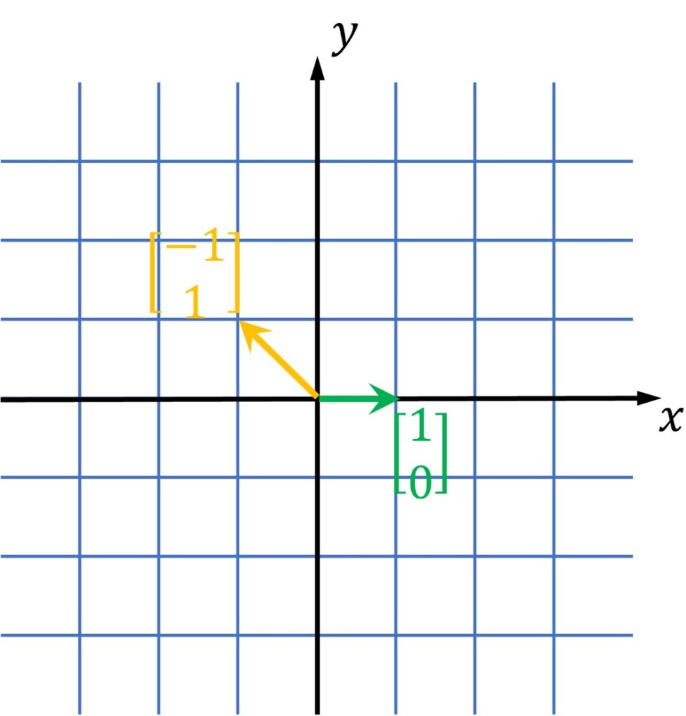
For instance, we can have a linear transformation giving me the following matrix and we can use eigenvectors as basis. So, the original transformation matrix has columns (3,0) and (1,2). We have calculated the eigenvectors: (1,0) and (-1,1).

So, that means that we can represent everything in this new coordinate system and we can go back. If we multiply it with the inverse, we would be able to have the complete equation given here:

At the end this will be our diagonal matrix.

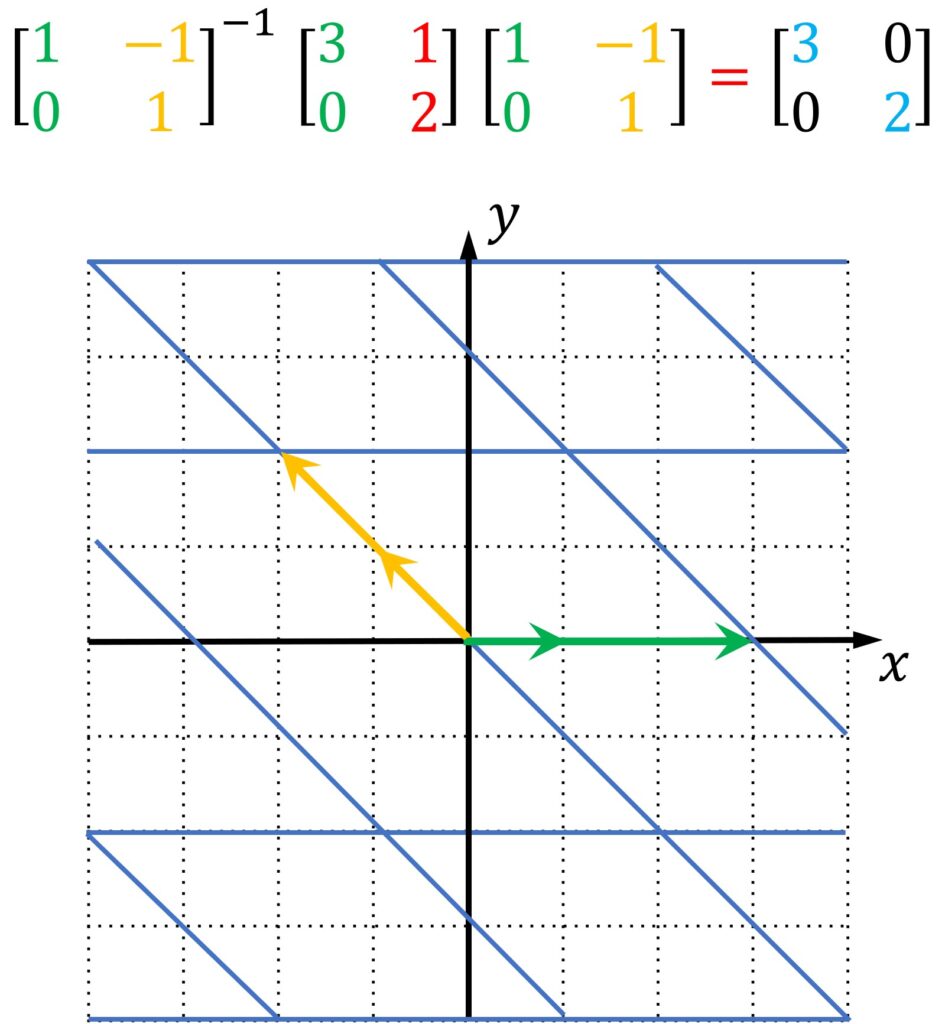
And once we have to work in such spaces where actually we know that our transformation matrix is diagonal that simplifies many things. For example, imagine that we need to calculate this hundreds of times. This matrix can be transformed in the eigen basis system so then it’s easy to compute the power of \(100 \) of a matrix in that, and then we can just go back to our original system and obtain our solution.

So, imagine that we have to multiply some vector with a matrix A 100 times. Then, we can go to an eigenvectors basis space. Multiplying a vector with a matrix A in a new space, will just scale it/stretch it. So, the result will be just multiplying with a diagonal matrix 100 times (very simple computationally). Then, the final vector we just move back to our original coordinate system and we have our solution.

Summary

Believe if or not we have finished. We do realize how important and interesting eigenvectors are in linear algebra. However, the real fun starts in the next post, where will be talking about Singular Value Decomposition (SVD). I you ask me (Vladimir), probably one of the top 10 most famous and influential algorithms in our history. So, SVD here we come.