#011 Developing a DCGAN for CelebA Dataset

Highlights: In the previous two chapters, we built two distinct DCGAN models, one for MNIST Handwritten Digit dataset, and the other for CIFAR-10 dataset.
In this chapter, we will build yet another DCGAN model. However, this time, we will use a different dataset known as the CelebA dataset. Let’s start by learning a bit about the CelebA dataset and its features.
Tutorial overview:
1. Downloading CelebA Dataset
The large-scale CelebFaces Attributes Dataset is a collection of over 200,000 images of celebrities. It is annotated in such a way that we get an understanding of what is happening in each image. Is the person wearing a hat? Is the person wearing glasses? Is the person smiling or not? And, so on.
You can download this dataset easily from Kaggle. Or, you can simply run the following code in ‘terminal’ or Google Colab.
!wget 'https://docs.google.com/uc?export=download&id=1q0iNpIa-sRq8k1LPgXGXX6YvQFPwQz5U&confirm=t' -O img_align_celeba.zipThe above command will download a zip file named img_align_celeba.zip. Let’s create a folder where we will unzip all of our images. We’ll name this folder celeba_dataset.
!mkdir celeba_datasetOnce the folder is created, we’ll simply unzip the zip file here.
!unzip -q img_align_celeba.zip -d celeba_dataset/img_align_celebaNow, inside this celeba_dataset folder, you will find another folder called img_align_celeba where all our images with respective filenames (ex: “202599.jpg”) will have been downloaded. This type of folder structure is necessary to work with the PyTorch image loader.
Let us use this dataset and start building our DCGAN model.
2. Initializing and Defining the DCGAN Model
The first thing we do is to import all the necessary and required libraries as shown in the code below.
import random
import matplotlib.pyplot as plt
import numpy as np

import torch
import torch.nn as nn
import torchvision
import torch.nn.functional as F
from torchvision import datasets
from torchvision import transforms
from torch.utils.data import DataLoader

# Set random seed for reproducibility
manualSeed = 999
#manualSeed = random.randint(1, 10000) # This will generate a random seed
print("Random Seed: ", manualSeed)
random.seed(manualSeed)
torch.manual_seed(manualSeed)

# Decide which device we want to run on
device = torch.device("cuda:0" if (torch.cuda.is_available()) else "cpu")
print(device)
We have given a particular value for the parameter manualSeed in the code above. You can choose to keep it as is and you will get identical results as ours. You can even set it manually or choose a random value. For this, you can ‘uncomment’ the line below it (refer to the code above).
Due to the proper structuring of folders, we will be able to load our data easily. The structuring was an important step because we will use the ImageFolder dataset class in our code. For this, we require subdirectories in the dataset’s root folder. The structure we have given meets all these requirements.
Now, we are ready to create the dataset. Let’s initiate the parameter dataLoader and let the program run so that we can visualize some of our training data.
transform = transforms.Compose([transforms.Resize(64),
                               transforms.CenterCrop(64),
                               transforms.ToTensor(),
                               transforms.Normalize((0.5, 0.5, 0.5), (0.5, 0.5, 0.5))])

# We can use an image folder dataset the way we have it setup.
# Create the dataset
dataset = datasets.ImageFolder(root="celeba_dataset/img_align_celeba",
                               transform=transform)
# Create the dataloader
data_loader = torch.utils.data.DataLoader(dataset, batch_size=128,
                                         shuffle=True, num_workers=2)
Have a look at how we sampled images from the dataset. The images can be seen below the code.
# Helper function, that takes a whole batch of images and shows them as a combined image
def imshow(img):
  npimg = img.numpy()
  plt.imshow(np.transpose(npimg, (1, 2, 0)))
  plt.show()

# We will take one batch of data and show the distribution of pixels in one sample image
data_iter = iter(data_loader)
images, labels = data_iter.next()

imshow(torchvision.utils.make_grid(images))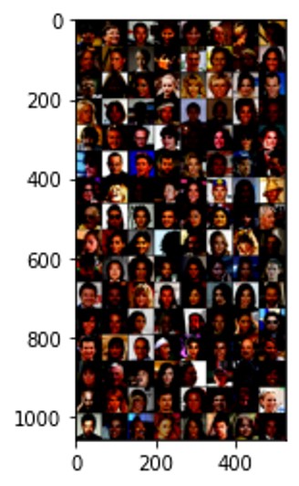
Weight Initialisation
With our input parameters set and the dataset prepared, we can now get into the implementation. We will start with the eight initialization strategies, and, then, talk about the generator, discriminator, loss functions, and training loop in detail.
In the DCGAN paper, the authors specify that all model weights should be randomly initialized from a Normal distribution with mean=0 and stdev=0.02. To meet these criteria, the weights_init function takes an initialized model as input and reinitializes all convolutional, convolutional-transpose, and batch normalization layers. This function is applied to the models immediately after initialization.
# Creating a function that will create a normal distribution of weights to the Convolutional layers
def init_normal(m):
classname = m.__class__.__name__
if classname.find('Conv') != -1:
nn.init.normal_(m.weight.data, 0.0, 0.02)
elif classname.find('BatchNorm') != -1:
nn.init.normal_(m.weight.data, 1.0, 0.02)
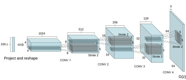
nn.init.constant_(m.bias.data, 0)Our goal is to convert a latent space, z, to a data space or RGB image of the same size as the training images (\(64 \times 64 \times 3 \)).
In practice, this is accomplished through a series of strided two-dimensional Convolutional Transpose layers, each paired with a 2D Batch Normalization layer and a ReLU activation.
Then, the output of the generator is fed through a tanh() function to return it to the input data range of [-1,1]. An image of the generator from the DCGAN paper is shown in the image below.
Defining the Generator Model
Now that we understand the architecture, we can write the code for the generator model. Note, that we will apply the weights_init function immediately after the initialization.
feature_map       = 64
latent_space_size = 100
class Generator(nn.Module):
    def __init__(self):
        super(Generator, self).__init__()

        self.convTranspose1 = nn.ConvTranspose2d( latent_space_size, feature_map * 8, 4, 1, 0, bias=False)
        self.convTranspose2 = nn.ConvTranspose2d( feature_map * 8  , feature_map * 4, 4, 2, 1, bias=False)
        self.convTranspose3 = nn.ConvTranspose2d( feature_map * 4  , feature_map * 2, 4, 2, 1, bias=False)
        self.convTranspose4 = nn.ConvTranspose2d( feature_map * 2  , feature_map * 1, 4, 2, 1, bias=False)
        self.convTranspose5 = nn.ConvTranspose2d( feature_map * 1  , 3              , 4, 2, 1, bias=False)

        self.bnorm1 = nn.BatchNorm2d(feature_map * 8)
        self.bnorm2 = nn.BatchNorm2d(feature_map * 4)
        self.bnorm3 = nn.BatchNorm2d(feature_map * 2)
        self.bnorm4 = nn.BatchNorm2d(feature_map * 1)

    def forward(self, x):
        x = self.convTranspose1(x)
        x = F.relu(self.bnorm1(x))

        x = self.convTranspose2(x)
        x = F.relu(self.bnorm2(x))

        x = self.convTranspose3(x)
        x = F.relu(self.bnorm3(x))

        x = self.convTranspose4(x)
        x = F.relu(self.bnorm4(x))

        x = self.convTranspose5(x)
        x = torch.tanh(x)
        return x

# Create the generator
generator = Generator().to(device)
Next, we create a function to generate the latent space z upon call and a random N number of vectors of the size 100.
# Helper function for creating a random latent vector
def generate_latent_vectors_z(N):
    z = torch.randn(N, 100, 1, 1, device=device)
    return z
We can even test the generator in the early stage, with no training, just by calling it on the latent space.
# Generate a random latent space of 100 elements which we will use to transform to an image
z = generate_latent_vectors_z(1).to(device)
random_noise = generator(z)

plt.imshow(random_noise[0].cpu().permute(1, 2, 0).detach().numpy())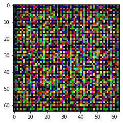
Defining the Discriminator Model
The next step is to build the discriminator, D. It is a binary classification network that takes an image as input and outputs a scalar probability that the input image is real (as opposed to fake).
Here, D takes a \(3 \times 64 \times 64 \) input image and processes it through a series of Conv2d, BatchNorm2d, and LeakyReLU layers, and outputs the final probability through a Sigmoid activation function.
class Discriminator(nn.Module):
    def __init__(self):
        super(Discriminator, self).__init__()
        self.conv1 = nn.Conv2d(3              , feature_map    , 4, 2, 1, bias=False)
        self.conv2 = nn.Conv2d(feature_map    , feature_map * 2, 4, 2, 1, bias=False)
        self.conv3 = nn.Conv2d(feature_map * 2, feature_map * 4, 4, 2, 1, bias=False)
        self.conv4 = nn.Conv2d(feature_map * 4, feature_map * 8, 4, 2, 1, bias=False)
        self.conv5 = nn.Conv2d(feature_map * 8, 1              , 4, 1, 0, bias=False)

        self.bnorm1 = nn.BatchNorm2d(feature_map*2)
        self.bnorm2 = nn.BatchNorm2d(feature_map*4)
        self.bnorm3 = nn.BatchNorm2d(feature_map*8)

        self.LeakyReLU = nn.LeakyReLU(0.2, inplace=True)
        self.sigmoid = nn.Sigmoid()

    def forward(self, x):
        x = F.leaky_relu(self.conv1(x))

        x = self.conv2(x)
        x = F.leaky_relu(self.bnorm1(x))

        x = self.conv3(x)
        x = F.leaky_relu(self.bnorm2(x))

        x = self.conv4(x)
        x = F.leaky_relu(self.bnorm3(x))

        x = self.conv5(x)
        x = self.sigmoid(x)
        return x
Defining the Loss Function
Now that we have set up the generator and the discriminator, we can specify how they learn through the loss functions and optimizers.
For the loss function, we will be using the Binary Cross Entropy Loss.
Then, we set up two separate optimizers, one for the discriminator and one for the generator. Both of these optimizers will be Adam Optimizers, each with a learning rate of 0.0002 respectively.
# Initialize BCELoss function
criterion = nn.BCELoss()

# Models
generator =     Generator().to(device)
discriminator = Discriminator().to(device)

# Use the modules apply function to recursively apply the initialization
generator.apply(init_normal)
discriminator.apply(init_normal)

# Optimizers
generator_optimizer     = torch.optim.Adam(generator.parameters(),     lr=0.0002)
discriminator_optimizer = torch.optim.Adam(discriminator.parameters(), lr=0.0002)
We have successfully initialized and defined our DCGAN model, including the generator, the discriminator, the loss function, and the optimizers. Now, we can start to train our model. We will first train our discriminator and then, train the generator.
3. Training the DCGAN Model
Similar to how we trained the DCGAN models for MNIST and CIFAR-10 datasets in the previous two posts, we will train this model in two legs:
- Training the Discriminator
- Training the Generator
Training the Discriminator
The goal of training the discriminator is to maximize the probability of correctly classifying a given input as real or fake.
We begin by constructing a batch of real samples from the training set. Then, we forward pass through the discriminator, calculate the loss, and calculate the gradients in a backward pass.
After this, we will construct a batch of fake samples with the current generator, forward pass this batch through the discriminator, calculate the loss, and accumulate the gradients with a backward pass.
Now, with the gradients accumulated from both the all-real and all-fake batches, we can optimize the Discriminator.
Training the Generator
As stated in the original paper, we want to train the generator by minimizing the loss to generate better fake images. It was actually proposed by Goodfellow to not provide sufficient gradients, especially, early on in the learning process.
We have to maximize the loss instead in order to fix this. In our code, we accomplish this by classifying the generator output from Part 1 with the discriminator, then, computing generators loss using real labels as GT, then, computing G’s gradients in a backward pass, and finally, updating G’s parameters with an optimizer step.
# Training Loop
print("Starting Training Loop...")
epochs = 20
N_samples = 128

# For each epoch
for epoch in range(epochs):
    # For each batch in the dataloader
    for idx, images in enumerate(data_loader):
        discriminator.zero_grad()

        if (idx%100 ==0):
            print(f"{epoch}/{epochs} epoch | {idx}/{len(data_loader)} batch \n")

        # Generate examples of real data
        real_data = images[0].to(device)
        real_data_label = torch.ones(real_data.shape[0]).to(device)

        # Training of Discriminator
        # Forward pass real batch through discriminator
        output = discriminator(real_data).view(-1)
        errD_real = criterion(output, real_data_label)
        # Calculate gradients for D in backward pass
        errD_real.backward()
        D_x = output.mean().item()

        # Create fake data with a generator
        z = generate_latent_vectors_z(len(real_data)).to(device)
        fake_data = generator(z)
        fake_data_label = torch.zeros(fake_data.shape[0]).to(device)

        # Forward pass fake data through discriminator
        output = discriminator(fake_data.detach()).view(-1)
        errD_fake = criterion(output, fake_data_label)
        errD_fake.backward()

        # Compute error of D as sum over the fake and the real batches
        errD = errD_real + errD_fake
        # Update discriminator
        discriminator_optimizer.step()

        # Training of Generator
        generator.zero_grad()
        real_data_label = torch.ones(fake_data.shape[0]).to(device) # fake labels are real for generator cost
        output = discriminator(fake_data).view(-1)
        errG = criterion(output, real_data_label)
        errG.backward()

        # Update Generator
        generator_optimizer.step()
When the network finishes training, we will save the generator and discriminator models.
torch.save(generator.state_dict(), '/content/DCGAN_celeba_g.pth')
torch.save(discriminator.state_dict(), '/content/DCGAN_celeba_d.pth')
Finally, we can now use our model to generate fake images with the help of the code snippet below.
# Generate a random latent space of 100 elements which we will use to transform to an image
z = generate_latent_vectors_z(len(real_data)).to(device)
fake_data = generator(z)
plt.imshow(fake_data[10].cpu().permute(1, 2, 0).detach().numpy())
Notice the result above. These images may not be perfect, but, in order to get accurate images, the models need to be trained on many more epochs. This means that you can experiment by setting the number of epochs to a more significant number to see how good the results get.
Another experiment that can be performed here is to modify this model by taking a different dataset and then, possibly, changing the size of the images as well as the model architecture.
Summary
Great! In no time, you have studied the workings and building of three interesting Deep Convolutional Generative Adversarial Network (DCGAN) models for three popular datasets – MNIST Handwritten Digit dataset, CIFAR-10 dataset, and CelebA dataset.
In the next post, we will go into detail about the working of a Generator model in DCGANs, especially, the input latent space, its mathematics, and a bit of code, of course.