#014 3D Face Modeling – Understanding primitives and transformations for image formation (Version B)

Highlight: Hi and welcome to our new post! In this post, we will continue our journey of understanding how fundamental computer vision techniques work. We first need to understand how images are formed, and how to go from a 3D scene to a 2D image. By understanding this we can develop models that mathematically formalize this process. So, let us start.
Understanding what are primitives
They represent the basic building blocks that are used to describe 3D shapes. For example, we will talk about points, lines, and planes which are the fundamental geometric building blocks.
2D Points
Let us start by exploring points. A point in 2D space can be written in inhomogeneous coordinates as follows:
$$ x = \begin{pmatrix} x \\ y \end{pmatrix} \in \mathbb{R}^2 $$
The point can be written in homogeneous coordinates as well, which takes the form of:
$$ \tilde{x} = \begin{pmatrix} \tilde{x} \\ \tilde{y} \\ \tilde{w} \end{pmatrix} \in \mathbb{P}^2 $$
Here we have extended the dimensionality of the vector space by one new dimension – \({w}\). For 2D points, this means that we have a 3D space. However, this space has a certain meaning. It is not just a 3D space, because we are removing the element at zero and we get a so-called projective space or \(\mathbb{P}^2\).
Note, whenever we see a tilde symbol over an element, we are looking at homogeneous coordinates and this way we differentiate between homogeneous and inhomogeneous coordinates.
Homogeneous vectors that differ only by scale are considered equivalent, and this is why it is effectively a 2D space because we define an equivalence class by all vectors that are related through a scaler operation. What does this mean?
Assume we have a vector \(\vec{a} = \{1, 1, 1\}\) and also a vector \(\vec{b} = \{2, 2, 2\}\), it is said that they fall into the same equivalence class. This means that homogeneous vectors are defined up to scale. This way of looking at homogeneous vectors allows us many things. For example, expressing points at infinity, the intersection of parallel lines, and expressing complex transformations very easily as concatenations of multiple transformations.
How can we go from a homogeneous space to an inhomogeneous space?
The first two elements of a homogeneous space represent the elements in the inhomogeneous space. So by making the third element a value of for example 1, we went from homogeneous to inhomogeneous coordinates. This new vector is called an augmented vector \(\bar{x}\). This augmented vector has a bar instead of a tilde symbol on top of it and it simply denotes it is a 3D vector with one particular element of the equivalence class, the element with value 1.
$$ \tilde{x} = \begin{pmatrix} \tilde{x} \\ \tilde{y} \\ \tilde{w} \end{pmatrix} = \begin{pmatrix} x \\ y \\ 1 \end{pmatrix} = \begin{pmatrix} x \\ 1 \end{pmatrix} = \tilde{x}$$
Now that we know how to go from homogeneous to inhomogeneous coordinates, the question arises, how do we go the opposite way?
$$ \bar{x} = \begin{pmatrix} x \\ 1 \end{pmatrix} = \begin{pmatrix} x \\ y \\ 1 \end{pmatrix} = \frac{1}{\tilde{w}}\tilde{x} = \frac{1}{\tilde{w}}\begin{pmatrix} \tilde{x} \\ \tilde{y} \\ \tilde{w} \end{pmatrix} = \begin{pmatrix} \tilde{x}/\tilde{w} \\ \tilde{y}/\tilde{w} \\ 1 \end{pmatrix} $$
To do this we just divide the elements by the last element from the homogeneous vector. There is also one special homogeneous vector, which is the so-called ideal points or points at infinity. These points are the points with the last element equal to zero. Looking at the equations above, these points cannot be represented as inhomogeneous coordinates, because dividing the elements with zero leaves us with an infinity vector. On the other hand, this leaves us with a way to conveniently express points that are located at infinity even without the need to use infinity symbols.
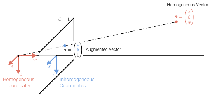
Above we can see a visual illustration of how the relationship looks between the two coordinates. We see a plane with the \(\tilde{w} = 1\) and we projected the 3D homogeneous coordinates to 2D inhomogeneous coordinates.
2D Lines
Using homogeneous coordinates we can also express lines, \(\tilde{l} = (a, b, c)^T\). We obtain the line equation if we take the inner product between the line and an augmented vector \(\bar{x}\).
$$ \{ \bar{x} | \tilde{l}\bar{x}=0 \} \Longleftrightarrow \{ x, y| ax + by + c = 0 \} $$
For all points, if the equation on the right has a value of zero, they are located on the line. Note, we can multiply the left-hand side of the equation arbitrarily and still obtain the line equation. One thing we can do is the normalization of the line so that:
$$ \tilde{l} = (n_x, n_y, d)^T = (n, d)^T $$
with \(||n||_2 = 1\). In this case, the \(n\) vector represents the normal vector perpendicular to the line and \(d\) is its distance to the origin.
One exception is the line at infinity \(\tilde{l}_\infty = (0, 0, 1)^T\) where the line passes through all the ideal points that we have defined earlier.
We can calculate the intersection of two lines by taking the cross product of the two lines.
$$ \tilde{x} = \tilde{l}_1 \times \tilde{l}_2$$
Also, the line joining two points can be written compactly as the first homogenous point cross-product the second point:
$$ \tilde{l} = \bar{x}_1 \times \bar{x}_2 $$
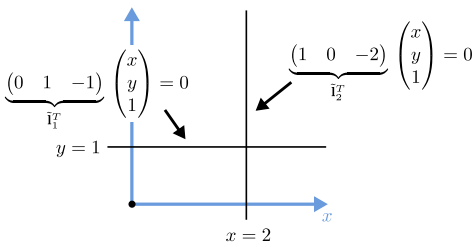
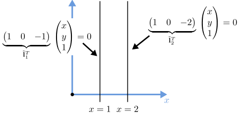
Let us see an example of how to calculate where two lines intersect. Suppose, we have two lines \(\tilde{l}_1^T\) and \(\tilde{l}_2^T\). The first line is characterized as \(x=2\) and the second as \(y=1\). To find the line vector, we need to find a vector that when multiplied with the augmented vector gives us a value of zero. Let us take a look at the equation below to understand how to calculate the vector for the first line.
$$ \begin{pmatrix} \tilde{x} & \tilde{y} & \tilde{w} \end{pmatrix} \begin{pmatrix} x \\ y \\ 1 \end{pmatrix} = 0 \Longrightarrow \begin{pmatrix} \tilde{x} & \tilde{y} & \tilde{w} \end{pmatrix} \begin{pmatrix} 0 \\ 1 \\ 1 \end{pmatrix} = 0 \Longrightarrow $$
out of which we get \(\tilde{x} = 0\), \(\tilde{y} = 1\), and \(\tilde{w} = -1\).
We do the same calculation for the second line.
In the plot below, visually we can see that they intersect at the point \((2, 1)\). Let us now see how we calculate this mathematically.
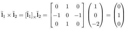
We can calculate this using the cross-product we referenced before. We create a cross-product matrix, which can be seen below, using the values from the first line.
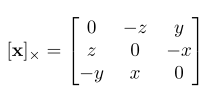
After we obtain this matrix we compute the cross-product between the matrix and the second line vector.
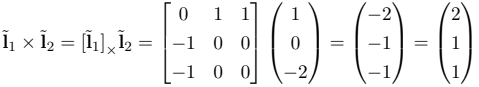
We can see that the values of this new point represent the correct intersection of these two lines. One question is, what happens when we have two parallel lines?
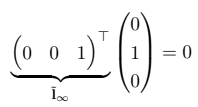
Similar to before we compute the cross-product for these two lines and we obtain the following results.
We see that the last element in the intersection point has a value of zero, meaning they intersect at infinity as expected. If we take the line at infinity and calculate the inner product with the intersection line, we get a value of zero. This means that the point in infinity actually lies on the line at infinity.
Complex algebraic objects
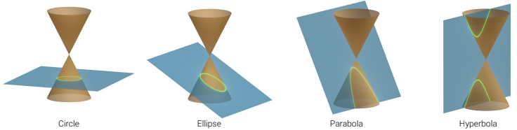
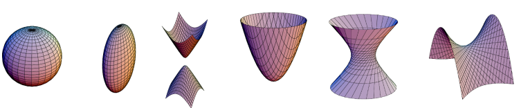
Using homogeneous equations we can express more complex algebraic objects. If we from the linear equation to polynomial equations, quadratic, we can express conic sections. A quadratic equation takes the form as follows:
$$ \{ \bar{x} | \bar{x}^T Q\bar{x} = 0 \}$$
The solution to this quadratic equation is a conic section. So, depending on how we orient the plane that can be seen below, it depends on the \(Q\) matrix, we get either a simple circle or ellipse or a parabola or hyperbola.
3D Points
Similarly, as for 2D points, we have our 3D points. They have both inhomogeneous coordinates
$$ x = \begin{pmatrix} x \\ y \\ z \end{pmatrix} \in \mathbb{R}^3 $$
and also homogeneous coordinates
$$ \tilde{x} = \begin{pmatrix} \tilde{x} \\ \tilde{y} \\ \tilde{z} \\ \tilde{w} \end{pmatrix} \in \mathbb{P}^3 $$
And we can go from homogeneous to inhomogeneous coordinates and vice versa.
3D Planes
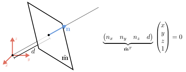
We can also represent planes as homogeneous coordinates \(\tilde{m} = (a, b, c, d)^T\).
$$ \{ \bar{x} | \tilde{m}^T \tilde{x} = 0 \} \Longleftrightarrow \{ x, y, z | ax+by + cz + d = 0 \} $$
Similar to the 2D lines we can normalize 3D planes. An exception is a plane at infinity that passes through all the ideal points for which \(\tilde{w} = 0\).
3D Lines
3D Lines are not as elegant to express as 3D planes and 2D lines. One way to represent them is to express points on a line as linear combinations of two points \(p\) and \(q\).
$$ \{ x | x = (1 – \lambda)p + \lambda q \bigwedge \lambda \in \mathbb{R} \}$$
This representation uses 6 parameters for 4 degrees of freedom.
3D Quadrics
The 3D analog of 2D conics is a quadratic surface.
$$ \{ \bar{x} | \bar{x}^TQ \bar{x} = 0 \} $$
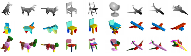
These quadrics are useful in the study of multi-view geometry and also serve as useful modeling primitives for modeling scenes of compact representation. For example, quadrics are used to create the objects in the figure[1] below.
2D Transformations
Now that we know the basic building blocks of objects, we can move on and see different transformations that can be applied to them. In this sub-section, we will cover the five most important types of transformations.
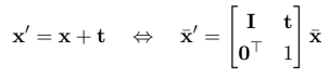
Translations – 2 degrees of freedom
Let us start with the simplest transformation, which is translation. Translations are used for shifting an object, in the image above we can see how this square was shifted from one location to another. This is given by just summing a translation vector with all the points of the square. This transformation preserves the orientation of the points.
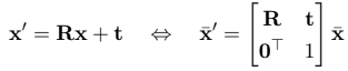
Euclidian transformation (Translation + Rotation) – 3 degrees of freedom
The second type of transformation is euclidian. It consists of two different transformations, a rotation, and a translation. We obtain the newly transformed coordinates by rotating our points using a rotation matrix \(R\) and then translating them by adding the \(t\) vector. The interesting thing about this type of transformation is that it preserves the lengths.
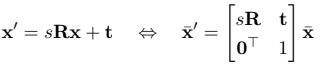
Similarity transformation (Translation + Scaled Rotation) – 4 degrees of freedom
The similarity transformation is a 2D translation, 2D rotation, and 2D scaling. It is the same as euclidian transformation, just scaling the points. This transformation preserves the angles between the lines.
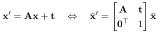
Affine transformations – 6 degrees of freedom
The rotation matrix has been replaced with a general arbitrary 2×2 matrix. Looking at the equation below, we have 4 DoF in the \(A\) matrix and 2 DoF in the \(t\) vector. This transformation preserves parallel lines.
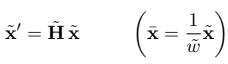
Perspective transformation – 8 degrees of freedom
The most general transformation that is defined with such a linear homogeneous equation is the perspective transformation or homography. Every point of a shape can transform into a different location and that is why we have 8 degrees of freedom. This transformation preserves the straight lines.
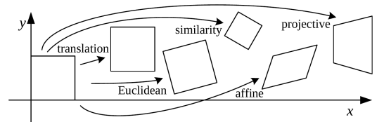
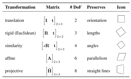
Overview of all the 2D transformations
On the image below, we can see a summary of all the transformations that can be applied to 2D objects.
Summary
We can now summarize have learned and seen in this post. We have seen what are 2D points/lines and 3D points/lines/planes and also seen some more complicated shapes in 2D and 3D. We have also explored different types of transformations that can be applied to 2D shapes and objects.
References
[1] Paschalidou, Ulusoy, and Geiger: Superquadrics Revisited: Learning 3D Shape Parsing beyond Cuboids. CVPR, 2019.