#010 Developing a DCGAN for CIFAR-10 Dataset

Strahinja Zivkovic GAN 05.09.2022 | 0

Highlights: In the previous post, we built a Deep Convolutional Generative Adversarial Network (DCGAN) for the MNIST Handwritten Digit Dataset. Taking forward the encouraging results we displayed in the previous chapter, let us build our first DCGAN model using the standard small image dataset, CIFAR-10.

By using a small and already well-understood dataset such as CIFAR-10, we can speed up the development and training of our model so that we are can focus more on the model architecture and the image generation process. As in the case of the previous post, we will gain a full understanding of how to define and train our discriminator and generator models, and use them to generate new images.

Tutorial overview:

Downloading the CIFAR 10 Dataset
Initializing and Defining the DCGAN Model
Training the DCGAN Model

1. Downloading the CIFAR-10 Dataset

The CIFAR-10 dataset consists of 60,000 colored (RGB) images of dimensions 3232 pixels divided into 10 classes (6,000 images per class).

The dataset is divided into five training batches and one test batch, each with 10,000 images. Have a look at the image below wherein we can see 10 classes of the dataset as well as 10 random images from each class.

Without further ado, let’s start by writing the code for our DCGAN model.

The first step is to import the necessary libraries.

import argparse
import os
import random
import torch
import torch.nn as nn
import torch.nn.parallel
import torch.backends.cudnn as cudnn
import torch.optim as optim
import torch.utils.data
import torchvision.datasets as dset
import torchvision.transforms as transforms
import torchvision.utils as vutils
import numpy as np
import matplotlib.pyplot as plt
import matplotlib.animation as animation
from IPython.display import HTML
from torchvision import datasets, transforms

# Set random seed for reproducibility
manualSeed = 999
#manualSeed = random.randint(1, 10000) # This will generate a random seed
print("Random Seed: ", manualSeed)
random.seed(manualSeed)
torch.manual_seed(manualSeed)
Code language: PHP (php)

Before we download the CIFAR-10 dataset, we need to convert the images from the dataset to PyTorch tensors. For this, we need to create a variable transform and apply the function transforms.ToTensor().

We can, now, automatically download the CIFAR-10 dataset by simply creating a variable using a simple string to specify the path.

Next, we create a training set. For this, we call the function CIFAR10(). As arguments to this function, we will provide data_path and set the train argument to True. This is because this part of the dataset will be used for training purposes. The third argument, download, is also set to True.

Then, with the same function, we will create an object, testset wherein our testing data will be stored. The only difference is that here, we will set the argument train to False. This means that this dataset will not be used for training purposes, but for testing.
After creating trainset and testset, we can create tarainloader and testloader.

transform = transforms.Compose(
    [transforms.ToTensor(),
     transforms.Normalize((0.5, 0.5, 0.5), (0.5, 0.5, 0.5))])
 
trainset = datasets.CIFAR10(root='./data', train=True,
                                        download=True, transform=transform)
trainloader = torch.utils.data.DataLoader(trainset, batch_size=128,
                                          shuffle=True, num_workers=2)
 
testset = datasets.CIFAR10(root='./data', train=False,
                                       download=True, transform=transform)
testloader = torch.utils.data.DataLoader(testset, batch_size=128,
                                         shuffle=False, num_workers=2)
 
classes = ('plane', 'car', 'bird', 'cat',
           'deer', 'dog', 'frog', 'horse', 'ship', 'truck')Code language: PHP (php)

Now, using the following function we can visualize our data.

# Helper function, that takes a whole batch of images and shows them as a combined image
def imshow(img):
  npimg = img.numpy()
  plt.imshow(np.transpose(npimg, (1, 2, 0)))
  plt.show()
 
# We will take one batch of data and show the distribution of pixels in one sample image
data_iter = iter(trainloader)
images, labels = data_iter.next()
imshow(torchvision.utils.make_grid(images))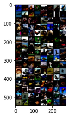Code language: PHP (php)

We will use the images in the training dataset as the basis for training a Generative Adversarial Network. Specifically, the generator model will learn how to generate new plausible photographs of objects using a discriminator that will, in turn, try to distinguish between real images from the CIFAR-10 training dataset and new images output by the generator model.

2. Initializing and Defining the DCGAN Model

Now that our dataset is downloaded and all prepared, we can start to implement our model. However, we need to initialize weights, to begin with.

Weight Initialisation

In the DCGAN paper, the authors suggested that all model weights should be randomly initialized using a Normal Distribution with mean=0, stdev=0.02.

Here, we will create a function weights_init that takes an initialized model as input and reinitializes all convolutional and batch normalization layers to meet this criterion. This function is applied to the models immediately after initialization.

# Creating a function that will create a normal distribution of weights to the Convolutional layers
def init_normal(m):
    classname = m.__class__.__name__
 
    if classname.find('Conv') != -1:
        nn.init.normal_(m.weight.data, 0.0, 0.02)
    elif classname.find('BatchNorm') != -1:
        nn.init.normal_(m.weight.data, 1.0, 0.02)
        nn.init.constant_(m.bias.data, 0)Code language: PHP (php)

Now that we have initialized the weights and the data has also been loaded, we can go on to define our models, starting with the discriminator.

Defining the Discriminator Model

Let’s quickly refresh the definition of a discriminator. A discriminator takes a sample image from our dataset as input and outputs a classification prediction as to whether the sample is real or fake. We call this a Binary Classification Problem. The discriminator model has a normal convolutional layer followed by three convolutional layers using a stride of 22 to downsample the input image.

The model has no pooling layers and a single node in the output layer with the sigmoid activation function to predict whether the input sample is real or fake.

The model is trained to minimize the Binary Cross-Entropy Loss Function, appropriate for Binary Classification. We will use some best practices in defining the discriminator model, such as the use of LeakyReLU instead of ReLU, using Dropout.

class Discriminator(nn.Module):
    def __init__(self):
        super(Discriminator, self).__init__()
        self.conv1 = nn.Conv2d(3              , feature_map    , 4, 2, 1, bias=False)
        self.conv2 = nn.Conv2d(feature_map    , feature_map * 2, 4, 2, 1, bias=False)
        self.conv3 = nn.Conv2d(feature_map * 2, feature_map * 4, 4, 2, 1, bias=False)
        self.conv4 = nn.Conv2d(feature_map * 4, feature_map * 8, 4, 2, 1, bias=False)
        self.conv5 = nn.Conv2d(feature_map * 8, 1              , 4, 1, 0, bias=False)
 
        self.bnorm1 = nn.BatchNorm2d(feature_map*2)
        self.bnorm2 = nn.BatchNorm2d(feature_map*4)
        self.bnorm3 = nn.BatchNorm2d(feature_map*8)
 
        self.LeakyReLU = nn.LeakyReLU(0.2, inplace=True)
        self.sigmoid = nn.Sigmoid()
 
    def forward(self, x):
        x = F.leaky_relu(self.conv1(x))
 
        x = self.conv2(x)
        x = F.leaky_relu(self.bnorm1(x))
 
        x = self.conv3(x)
        x = F.leaky_relu(self.bnorm2(x))
        
        x = self.conv4(x)
        x = F.leaky_relu(self.bnorm3(x))
 
        x = self.conv5(x)
        x = self.sigmoid(x)
        return x

Defining the Generator Model

The generator model is responsible for creating new, fake, yet plausible, small photographs of objects. It does this by taking a point from the latent space as input and outputting a square color image.

The latent space is an arbitrarily defined vector space of Gaussian-distributed values, e.g. 100 dimensions. It has no meaning. However, if we draw points from this space randomly and provide them to the generator model during training, the generator model will assign meaning to the latent points. In turn, the latent vector space represents a compressed representation of the output space, till the end of the training. These CIFAR-10 images can be turned into plausible CIFAR-10 images with the help of our generator.

In order to do this, we use the ConvTranspose2d()function, to transpose the Convolutional layer.

Usually, a z vector is of a much lower dimension than the output image. Thus, this information will propagate throughout the network and the output will have the dimension of the original images from a dataset. Therefore, using the Transpose Convolutional layer, we apply an upsampling process and use a stride of 22.

In the final layer, we will use the tanh() activation function. This will produce the output image with pixel intensity values in the interval of [-1,1]. Hence, the images from the original CIFAR-10 dataset should also be rescaled to match this interval such that we have a standardized input into our discriminator.

In addition to a Transpose Convolutional layer, we will use Batch Normalization layers represented by the function BatchNorm2d().

feature_map       = 64
latent_space_size = 100
 
class Generator(nn.Module):
    def __init__(self):
        super(Generator, self).__init__()
 
        self.convTranspose1 = nn.ConvTranspose2d( latent_space_size, feature_map * 8, 4, 1, 0, bias=False)
        self.convTranspose2 = nn.ConvTranspose2d( feature_map * 8  , feature_map * 4, 4, 2, 1, bias=False)
        self.convTranspose3 = nn.ConvTranspose2d( feature_map * 4  , feature_map * 2, 4, 2, 1, bias=False)
        self.convTranspose4 = nn.ConvTranspose2d( feature_map * 2  , feature_map * 1, 4, 2, 1, bias=False)
        self.convTranspose5 = nn.ConvTranspose2d( feature_map * 1  , 3              , 4, 2, 1, bias=False)
 
        self.bnorm1 = nn.BatchNorm2d(feature_map * 8)
        self.bnorm2 = nn.BatchNorm2d(feature_map * 4)
        self.bnorm3 = nn.BatchNorm2d(feature_map * 2)
        self.bnorm4 = nn.BatchNorm2d(feature_map * 1)
 
    def forward(self, x):
        x = self.convTranspose1(x)
        x = F.relu(self.bnorm1(x))
 
        x = self.convTranspose2(x)
        x = F.relu(self.bnorm2(x))
 
        x = self.convTranspose3(x)
        x = F.relu(self.bnorm3(x))
 
        x = self.convTranspose4(x)
        x = F.relu(self.bnorm4(x))
 
        x = self.convTranspose5(x)
        x = torch.tanh(x)
        return x

Defining the Loss Function

Now that we have defined our generator and discriminator neural networks, our next step would be to define the loss function. And, for this, we will use the Binary Cross-Entropy Loss Function.

For this, we set up two separate optimizers, one for the discriminator and one for the generator, and initiate the learning rate with the value of 0.0002.

# Initialize BCELoss function
criterion = nn.BCELoss()
 
# Models
generator =     Generator().to(device)
discriminator = Discriminator().to(device)
 
# Use the modules apply function to recursively apply the initialization
generator.apply(init_normal)
discriminator.apply(init_normal)
 
# Optimizers
generator_optimizer = torch.optim.Adam(generator.parameters(),     lr=0.0002)
discriminator_optimizer = torch.optim.Adam(discriminator.parameters(), lr=0.0002)Code language: PHP (php)

There we go! We have successfully initialized and defined our model including the discriminator, the generator, and the loss function. Let’s move ahead to the next step of our implementation, where we will train our models.

3. Training the DCGAN Model

After initializing the weights and defining our discriminator, generator, and loss function, we are ready to train our model. There are two legs to training the model:

Training the Discriminator
Training the Generator

Let’s first understand the training process as a whole. Essentially, in the training process, the generator and the discriminator are playing a minimax game. In simple words, the generator is trying to create images that actually fool the discriminator and the discriminator is always trying to be right. In this minimax game, they try to exploit the weaknesses of their adversary and at the same time, they are forced to fix their own weaknesses.

This minimax game between the generator and the discriminator can be expressed using the following equation:

$$ \min _G \max _D \mathbb{E}_{x \sim q_{\text {data }}(\boldsymbol{x})}[\log D(\boldsymbol{x})]+\mathbb{E}_{\boldsymbol{z} \sim p(z)}[\log (1-D(G(\boldsymbol{z})))] $$

You can read more about this minimax game by checking out this blog post.

Training the Discriminator

As mentioned earlier, the primary goal of training the discriminator is to classify a given input image as real or fake. In other words, we need to maximize the probability that a given input is a real image.

To do this, we will first construct a batch of real samples from the training set. Then, we will conduct a forward pass through the discriminator and calculate the loss. After that, we will conduct a backward pass and calculate the gradients.

We keep applying the same steps for the fake samples as well. In this way, we accumulate the gradients from both the real and fake batches.

Once we are done with the training of the discriminator, we can move on to training the generator.

Training the Generator

In order to train the generator, we need to maximize an objective function such that we can get the perfect discriminator. However, the goal of the generator is to fool the discriminator as much as it can. Hence, it will try to do the opposite, i.e., to minimize the objective function.

$$ \log (D(G(z))) \rightarrow \min $$

In practice, this means that the term $\log (1-\log (D(G(z)))) $ is as small as possible. This makes sense, as we want to fool the discriminator.

So, essentially, we want the term $D(G(z)) $ to be as close as possible to 1. In this way, we can minimize the term $\log (1-\log (D(G(z)))) $ and help the generator reach its goal.

To actually accomplish this, we will classify the generator output from the first part with the discriminator, compute generator loss using real labels as ground truth, compute generator gradients in a backward pass, and finally, update generator parameters with an optimizer step.

# Helper function for creating a random latent vector
def generate_latent_vectors_z(N):
    z = torch.randn(N, 100, 1, 1, device=device)
    return z    



# Training Loop
print("Starting Training Loop...")
epochs = 20
N_samples = 128
 
# For each epoch
for epoch in range(epochs):
    # For each batch in the dataloader
    for idx, images in enumerate(trainloader):
        discriminator.zero_grad()
 
        if (idx%100 ==0):
            print(f"{epoch}/{epochs} epoch | {idx}/{len(trainloader)} batch \n")
 
        # Generate examples of real data
        real_data = images[0].to(device)
        real_data_label = torch.ones(real_data.shape[0]).to(device)
 
        # Training of Discriminator
        # Forward pass real batch through discriminator
        output = discriminator(real_data).view(-1)
        errD_real = criterion(output, real_data_label)
        # Calculate gradients for D in backward pass
        errD_real.backward()
        D_x = output.mean().item()
 
        # Create fake data with a generator
        z = generate_latent_vectors_z(len(real_data)).to(device)
        fake_data = generator(z)
        fake_data_label = torch.zeros(fake_data.shape[0]).to(device)
 
        # Forward pass fake data through discriminator
        output = discriminator(fake_data.detach()).view(-1)
        errD_fake = criterion(output, fake_data_label)
        errD_fake.backward()
 
        # Compute error of D as sum over the fake and the real batches
        errD = errD_real + errD_fake
        # Update discriminator
        discriminator_optimizer.step()
 
        # Training of generator
        generator.zero_grad()
        real_data_label = torch.ones(fake_data.shape[0]).to(device) # fake labels are real for generator cost
        output = discriminator(fake_data).view(-1)
        errG = criterion(output, real_data_label)
        errG.backward()
 
        # Update Generator
        generator_optimizer.step()
 
 
torch.save(generator.state_dict(), '/content/DCGAN_celeba_g.pth')
torch.save(discriminator.state_dict(), '/content/DCGAN_celeba_d.pth')
Code language: PHP (php)

Now that we have trained our model, we can make some fake images using the generator. We generate a random latent vector and pass it through the generator.

# Generate a random latent space of 100 elements which we will use to transform to an image
z = generate_latent_vectors_z(len(real_data)).to(device)
fake_data = generator(z)
plt.imshow(fake_data[10].cpu().permute(1, 2, 0).detach().numpy())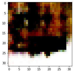Code language: PHP (php)

Remember, to achieve better results, always train your model for more epochs. So, after 100 epochs, if the model remains stable, you will see start seeing improvement in the generated images.

Summary

Well, that’s good progress that we made in this post. Now, we have built two DCGAN models, one using the MNIST Handwritten Digit dataset and the other using the CIFAR-10 dataset. In the next post, we will learn to build more models using various other datasets.

#010 Developing a DCGAN for CIFAR-10 Dataset