#009 Developing a DCGAN for MNIST Dataset

Strahinja Zivkovic GAN 05.09.2022 | 0

Highlights: In the previous posts we have already explored the basic GAN idea, and we have studied the guidelines for more stable training. In particular, we have analyzed the “GAN Hacks” in post 007 that was proposed in a DCGAN paper. In addition, we have implemented a simple GAN network to learn the mapping of a 1D function.

Hence, to prove that the GANs are a promising family of generator architecture, we need to start with more challenging examples. Therefore, in this post, we will show how GAN (or DCGAN model) can be trained so that we generate meaningful representatives of handwritten digits. That is, we will learn how to create new samples that will resemble the MNIST dataset. So, let’s begin.

Tutorial Overview:

Downloading MNIST Handwritten Digit Dataset
Training the Discriminator
Training the Generator
Generating Training Dataset
Training the DCGAN Model

1. Downloading MNIST Handwritten Digit Dataset

Before we proceed with GANs we will start with a simple, yet important step. We are going to show you how to download the MNIST dataset and explore some of its properties in PyTorch. Probably, you have already most likely worked with this, so you can go quickly through this paragraph.

The Modified National Institute of Standards and Technology (MNIST) dataset is a collection of 60,000 little square grayscale photos of handwritten single numbers ranging from 0 to 9. Commonly, it is used for classification where the goal is to classify a handwritten image presented to you. Every image is labeled with the corresponding class label.

Now, let’s start by importing the necessary libraries.

import torch 
import torch.nn as nn
from torchvision import datasets
import torchvision
import matplotlib.pyplot as plt
import numpy as np
from torchvision import transforms
from torchvision.transforms.transforms import NormalizeCode language: JavaScript (javascript)

To automatically download the MNIST dataset we can use the torchvision module. First, we will create a list of transforms that we want to compose called transform and apply a method torchvision.Compose(). First, we will call the function transforms.ToTensor() which will convert the entire data into a torch.tensor data structure. Second, we will also call the method transforms.Normalize() and pass as arguments pre-calculated values of the global mean and standard deviation of the MNIST dataset.

transform = transforms.Compose([transforms.ToTensor(),
                                transforms.Normalize([0.1307], [0.3081])])

With this code snippet, we have converted the PIL image data format into a tensor data structure, and also normalized the images.

Next, we will create variable data where we will download the MNIST dataset using the function datasets.MNIST(). As arguments, we will provide the root where we have specified the folder where the dataset will be downloaded; we will set the train to True because this part of the dataset will be used for training purposes. The third argument is the download which is also set to True. Finally, in order to convert the data to tensors, we will set the parameter transform=transform.

Since we are working with a large number of parameters it is always useful to load data in batches using the DataLoader class. So, we will create a variable data_loader and call torch.utils.data.DataLoader() function. As the first argument, we will pass a name of a dataset variable. Then, we will set the second argument batch_size to be equal to 128. The third parameter is shuffle which will shuffle our data after we pass the boolean value of True.

To speed up the training process, we can use the argument num_workers. It is an optional attribute of the DataLoader class which specifies how many sub-processes we want to use for data loading. In our case, we will set this argument to be equal to 2.

# load the MNIST dataset using a torchvision module
data = datasets.MNIST(root = './' , train=True, transform=transform, download=True)
data_loader = torch.utils.data.DataLoader(data, batch_size=128,
                                         shuffle=True, num_workers=2)Code language: PHP (php)

In order to iterate through our data, we call the function iter() and pass the data_Loader variable as an argument. After that, we will initialize the first batch using the command .next().

dataiter = iter(trainLoader)
images, labels = dataiter.next()

To display the images we will define the function imshow(). This function will normalize the images, transform them into NumPy arrays, and reorder the channels. Then, we will call the imshow() function and as an argument, we will pass torchvision.utils.make_grid(images). In that way, we will make a grid of all images in a single batch from the MNIST dataset.

def imshow(img):
  img = img / 2 + 0.5
  npimg = img.numpy()
  plt.imshow(np.transpose(npimg, (1, 2, 0)))
  plt.show()
 
imshow(torchvision.utils.make_grid(images))

We can also check the labels of these images from the batch.

print(labels)Code language: PHP (php)

tensor([0, 4, 8, 0, 2, 3, 8, 1, 5, 9, 0, 7, 5, 9, 9, 2, 0, 7, 4, 0, 2, 4, 6, 9,
        3, 5, 1, 3, 5, 3, 7, 1, 0, 2, 5, 0, 3, 9, 3, 7, 2, 9, 1, 0, 3, 3, 7, 5,
        6, 2, 8, 1, 9, 4, 5, 4, 7, 8, 5, 8, 3, 9, 0, 1, 6, 9, 6, 3, 5, 5, 1, 2,
        3, 5, 6, 0, 3, 1, 5, 5, 9, 6, 4, 5, 0, 0, 5, 3, 5, 9, 1, 9, 8, 2, 4, 0,
        5, 3, 4, 0, 5, 5, 8, 9, 8, 1, 5, 0, 2, 5, 2, 5, 5, 5, 4, 0, 3, 5, 9, 1,
        8, 8, 5, 2, 5, 8, 0, 7])

2. Training the Discriminator

The discriminator model’s goal is to classify the image correctly. Therefore, it will get both fake and real images as input.

The input image will be of size \(28\times 28 \).
And, the output will be a probability score in the interval \([0,1] \).

We will implement the discriminator according to the DCGAN paper. Thus, we will follow most of the rules and hacks that we have already explained in Chapter 7, but our neural networks will be much simpler in this chapter.

We will be using the standard convolutional layers (Conv2d) and batch normalization layers (BatchNorm2d) as recommended. For the optimisation purpose, we will use the Adam Optimisation Algorithm. Finally, recall that for the DCGAN model use of the LeakyReLU activation function is recommended with a value of 0.2 as the slope coefficient.

Have a look at the following code snippet that efficiently implements the discriminator network.

# Creating the discriminator model ( Goal: Discriminate wether an image is real or not )
class Discriminator(nn.Module):
    def __init__(self):
        super(Discriminator, self).__init__()
        self.conv1 = nn.Conv2d(1, 64, kernel_size=(3,3), stride=(2,2), padding=1, bias=False)
        self.LeakyReLU = nn.LeakyReLU(0.2)
        self.conv2 = nn.Conv2d(64, 64, kernel_size=(3,3), stride=(2,2), padding=1, bias=False)
        # since we are using a stride of (2,2) in both Conv2d layers
        # the feature map will shrink to 28 --> 14 --> 7
        self.linear = nn.Linear(7*7*64, 1)
        self.sigmoid = nn.Sigmoid()
        
    def forward(self, x):
        x = self.conv1(x)
        x = self.LeakyReLU(x)
        x = self.conv2(x)
        x = self.LeakyReLU(x)
        x = torch.flatten(x, 1)
        x = self.linear(x)
        x = self.sigmoid(x)
        return x

Next, we will create a discriminator model D. We will take the first image from the MNIST dataset being stored in our variable data[0][0]. Just as a reminder, the first [0] we use to index the image element in a dataset, and the second [0] we use to access the image, as the images are stored as tuple pairs (image, label).

D = Discriminator()
# Sanity check 
test_image = data[0][0]
test_image = test_image.unsqueeze(0)
D(test_image)Code language: PHP (php)

tensor([[0.5232]], grad_fn=<SigmoidBackward0>)Code language: HTML, XML (xml)

D.parametersCode language: CSS (css)

<bound method Module.parameters of Discriminator(
  (conv1): Conv2d(1, 64, kernel_size=(3, 3), stride=(2, 2), padding=(1, 1), bias=False)
  (LeakyReLU): LeakyReLU(negative_slope=0.2)
  (conv2): Conv2d(64, 64, kernel_size=(3, 3), stride=(2, 2), padding=(1, 1), bias=False)
  (linear): Linear(in_features=3136, out_features=1, bias=True)
  (sigmoid): Sigmoid()
)>
Code language: HTML, XML (xml)

The final hack that we will apply to the discriminator is to initialize weights using a Gaussian normal distribution.

# Creating a function that will create a normal distribution of weights to the Convolutional layers
def init_normal(m):
    if type(m) == nn.Conv2d:
        nn.init.normal_(m.weight, 0., 0.02)
 
# Use the modules apply function to recursively apply the initialization
D.apply(init_normal)Code language: PHP (php)

Discriminator(
  (conv1): Conv2d(1, 64, kernel_size=(3, 3), stride=(2, 2), padding=(1, 1), bias=False)
  (LeakyReLU): LeakyReLU(negative_slope=0.2)
  (conv2): Conv2d(64, 64, kernel_size=(3, 3), stride=(2, 2), padding=(1, 1), bias=False)
  (linear): Linear(in_features=3136, out_features=1, bias=True)
  (sigmoid): Sigmoid())
Code language: PHP (php)

3. Training the Generator

While discriminator nicely fits into a classic deep learning architecture, the generator neural network is a new and exciting part of the GAN. In essence, it is also the neural network, but its architecture more resamples decoder architectures. Hence, the generator’s goal is to create realistic replicas of the images from the MNIST dataset.

To achieve this, the generator has:

As input, a latent vector \(z \)of a lower dimension where \(z=100 \)
As output, we have a (realistic) fake image that is modeled according to the original dataset

For this, we do use a Transpose Convolutional layer (ConvTranspose2d()). Commonly, a z vector is of a much lower dimension than the output image. Thus, this information will propagate throughout the network and the output will have the dimension of the original images from a dataset. Therefore, we need to use an upsampling process, which here we achieve with Transpose Convolution and the use of a stride =(2,2).

At the final layer, we will use the Tanh() activation function. This will produce the output image with pixel intensity values in the interval of [-1,1]. Hence, the images from the original MNIST dataset should also be rescaled to match this interval, so that we have a standardized input into our discriminator.

In addition, we will use Batch Normalisation layers (BatchNorm2d()). Moreover, here we will use an LeakyReLU activation function, with a slope coefficient of 0.02.

The model itself is implemented with the following code:

# Creating the generator model ( Goal: generate fake images )
class Generator(nn.Module):
    def __init__(self):
        super(Generator, self).__init__()
        self.n_dim = 7 * 7 * 128 
        # here we use a hardcoded value of dimnsionality for our latent z vector ( 100 )
        self.fc1 = nn.Linear( 100, 128 * 7 * 7 )
        self.convTranspose1 = nn.ConvTranspose2d(128, 128, kernel_size=(4,4), stride = (2,2), padding=0)
        self.leaky = nn.LeakyReLU(0.2)
        self.conv2d = nn.Conv2d(128, 1, kernel_size = (7,7), stride = (1,1), padding = 0)
    
    def forward(self, x):
        x = self.fc1(x)
        x = self.leaky(x)
        x = x.view(-1,128 ,7,7)
        x = self.convTranspose1(x)
        x = self.leaky(x)
        x = self.convTranspose1(x)
        x = self.leaky(x)
        x = self.conv2d(x)
        x = torch.tanh(x)
        return x

Note, that here, we do use a Dense (fully connected) layer, to resize the original latent vector z. We have set a dimension of z=100, and therefore, we are resizing it (x = x.view(-1,128,7,7)) to a size that can be remapped for 2D transpose convolutional layers.
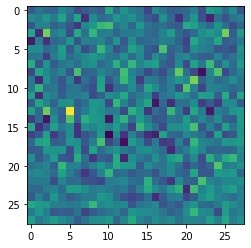
Before proceeding further, we will just do a sanity check. We will initialize the generator object. Next, we will pass the desired input and we will plot the fake image produced by the generator. Obviously, the weights of the generator are still randomly initialized, so the output image represents noise. The data from the generator are in the form: \(batch \times channel \times height \times width \). Therefore, to be able to plot the image, we will .squeeze(0) the generated tensor two times.

# sanity check 
G = Generator()
# Generate a random latent space of 100 elements which we will use to transform to an image
z = torch.randn(100)
x_hat = G(z)
plt.imshow(x_hat.squeeze(0).squeeze(0).detach().numpy())
Code language: PHP (php)

4. Generating Training Dataset

Here, we will re-engineer a part of the code for fake data generation. Note that this part will be very similar to the one already developed in chapter 6. Since the fake data generation requires only a random variable z, which is an input to the generator, we only need to make sure that we specify the dimension of a z correctly. In this experiment, we have decided to use a value of dim{z}=100. Then, we will use sampling from a Ggaussian distribution (torch.randn()) and we will generate the batch size (N).

# Helper function for creating a random latent vector
def generate_latent_vectors_z(N):
    z = torch.randn(N, 100)
    return z


# Creates fake latent vectors, passes them through the generator
# Returns the newly generated images with 0's as labels, indicating they are fake images
def generate_fake_samples(G, N):
    z = generate_latent_vectors_z(N)
    x_fake = G(z)
    y_fake = torch.zeros(N,1)
    return x_fake, y_fake
Code language: PHP (php)

Note, that along with the x_fake generated images, we will also output the y_fake as a vector of zeros.

These functions we will use during a training process to generate the fake data. The real data we will use directly from the MNIST dataset. A convenient approach is just to load them from the dataloader variable in batches. However, we have checked that the pixel intensity values in the dataset are set to the interval [0,1]. On the other hand, the output from the generator is Tanh().

As we can see this output generates fake images with the pixel intensity values from [-1,1]. Therefore, we will rescale the original image data from [0,1] to [-1,1]. Here is a simple function to achieve this:

def rescale_image_batch(image):
    # we assume that the original MNIST dataset is in the interval [0, 1]
    image = image - 0.5
    image = image * 2
    return imageCode language: PHP (php)

Hence, during the training phase, we will just call this function and rescale the real dataset.

5. Training the DCGAN Model

In the process of training, we will first train our generator model and then the discriminator, this is because the generator needs a head start in order for it to generate better images. We will iterate through the epochs defined and also print information about the training at every 100 batches.

epochs = 2  
 
# Models
generator =     Generator()
discriminator = Discriminator()
 
generator.apply(init_normal)
discriminator.apply(init_normal)
 
# Optimizers
Generator_optimizer = torch.optim.Adam(generator.parameters(),     lr=0.001)
discriminator_optimizer = torch.optim.Adam(discriminator.parameters(), lr=0.001)
 
# loss
loss = nn.BCELoss()
 
N = 128
 
for i in range(epochs):
    for idx, images in enumerate(data_loader):
        generator_optimizer.zero_grad()
        if (idx%100 ==0):
            print(f"{i}/{epochs} epoch | {idx}/{len(data_loader)} batch \n")
 
        # Create a fake data with a generator
        fake_data, fake_data_label = generate_fake_samples(generator, N)
        # here we define the INVERSE labels for fake data
        fake_data_label = torch.ones(N,1)
 
        # Generate examples of real data
        real_data =images[0]
        real_data = rescale_image_batch(real_data)
        real_data_label = torch.ones(real_data.shape[0],1)
 
        # Train the generator
        # We invert the labels here and don't train the discriminator because we want the generator
        # to make things the discriminator classifies as true.
        generator_discriminator_out = discriminator(fake_data)
        generator_loss = loss(generator_discriminator_out, fake_data_label)
        generator_loss.backward()
        generator_optimizer.step()
 
        # Train the discriminator on the true/generated data
        discriminator_optimizer.zero_grad()
        true_discriminator_out = discriminator(real_data)
        true_discriminator_loss = loss(true_discriminator_out, real_data_label)
 
        # see our post about AUTOGRAD
        generator_discriminator_out = discriminator(fake_data.detach())
        generator_discriminator_loss = loss(generator_discriminator_out, torch.zeros(N,1))
        discriminator_loss = (true_discriminator_loss + generator_discriminator_loss) / 2
        discriminator_loss.backward()
        discriminator_optimizer.step()
Code language: PHP (php)

When the model finishes its training we can use the generator to generate images. We will show the last image the model has generated, it should also be the best-generated image.

imshow(torchvision.utils.make_grid(fake_data[:4]))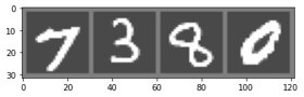Code language: CSS (css)

As you can see, our model created pretty realistic images.

Summary

In this post, we have learned how the DCGAN model can be trained on the MNIST Handwritten Digit Dataset. In the next post, we are going to build our first DCGAN model using the standard small image dataset, CIFAR-10.

#009 Developing a DCGAN for MNIST Dataset