#008 The Mathematics of GANs

Highlights: In the previous posts, we brushed the surface of our book’s hero concept of Generative Adversarial Networks (GANs). We also learned about training stable GANs using Deep Convolutional Generative Adversarial Networks (DCGANs).

In this post, we will dive a little bit more into the details of the GANs. We will observe their mathematical foundations through the fundamentals of probability and optimization methods. So, let’s begin.

Tutorial overview:

1. Adversarial Learning
2. The Adversarial Game
3. Loss Function and Optimisation
4. Optimal Solution of GAN
5. Architectures of the Discriminator and Generator

1. Adversarial Learning

We will start this post by explaining adversarial learning and the Vanilla GAN as explained in [1].

One way of interpreting GANs is that we start with a Generator. Commonly, it is designed as a deep neural network.

Next, imagine that the generator’s goal is to make fake money bills. Then, they will be judged by a human expert visually to determine if they are counterfeit or not. 

This is the initial idea. But, we cannot include humans to judge automatic algorithms. Hence, we will have another model, which is also a neural network and its goal would be to judge whether the input money bill is real or fake. This neural network is called Discriminator.

There is nothing new or special with a discriminator. It is a neural network with a commonly used binary cross-entropy loss. Next, the inputs to the generator are both real and fake images. Naturally, the goal of the discriminator is to classify the bills and to achieve the highest possible accuracy. 

At the beginning of the training, both networks will have their weights set to zero. This means that both the generator and the discriminator will perform poorly. This is in particular true for the generator whose fake samples will be really easy to classify correctly. However, both networks are trained in parallel. While we train the generator network, the discriminator parameters are kept fixed and vice-versa. Hence, we proceed with the training simultaneously.

Later we will see that this concept of training is called a minimax game. Both networks actually compete with each other and they are getting better and better.

The end of the game happens when we reach an equilibrium. At this point, at least theoretically, the discriminator will not be able to distinguish between real and fake images.

2. The Adversarial Game

The original GAN was proposed by Ian Goodfellow in his paper in 2014 [2]. We can refer to this neural network architecture and mechanism as Vanilla GAN.

Now, assume that we have a \(d \) – dimensional dataset with \(n \) data points: 

$$ \left\{x_i \in \mathbb{R}^d\right\}_{i=1}^n $$

In GAN, we have a generator \(G \) such that \(G: z \rightarrow x \), where \(G(z)=x \).

Here, a distribution \(z \sim p_z(z) \) is a random noise (e.g. Gaussian or Normal distribution).

Next, from this noise, we create an image \(x \). The goal of generator \(G \) is to produce images \(x \) that are as similar as possible to the image x from the original dataset (true data images). 

In addition to the generator network, we also have a discriminator. In essence, it is a simple binary classifier with the sigmoid activation function that finally maps an input image into the interval \([0,1] \) as follows.

$$ D: x \rightarrow[0,1] $$

Here, we assume that the discriminator value 1 will represent that x comes from the real or true dataset of images, whereas value 0 represents the fake generated image.

This is a supervised classification problem that assumes that the data are labeled. However, here we do not have a human to perform the labeling. Class 0 simply means that the image is created from a generator, whereas class 1 is assigned to every true image from the original dataset. Therefore, we have the following mapping:

$$ D(x):= \begin{cases}1 & \text { if } x \text { is real } \ 0 & \text { if } x \text { is generated (fake) }\end{cases} $$

Hence, the ideal discriminator will output 1 for every true image, whereas it will output 0 for a fake image. In practice, the output values will be in the interval \([0,1] \).

In case the discriminator is fooled by the generator, it means that it has started to produce images of very good quality, and hence, the job of the discriminator becomes quite challenging. In practice, this means that the human can also miss recognizing that the generated image is a fake one. For instance, we can have a highly photorealistic face image of a “person that does not exist”. 

3. Loss Function and Optimisation

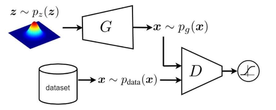
In GAN literature, the distribution of the real data and the noise that we use for image generation is denoted by \(p_{\text {data }}(x) \) and \(p_{\text {z }}(z) \) respectively. This is depicted in the image below. By default, the dataset consists of samples that have a distribution \(p_{\text {data }}(x) \). On the other hand, a generator outputs fake images that are created using a random noise z. A common choice to model the noise is to assume that it has Gaussian or normal distribution.

The two networks are trained simultaneously. In particular, the objective is optimized as a minimax optimization problem that is solved using alternate optimization until convergence is reached. The following loss function is used for vanilla GAN:

$$ \begin{array}{rl}\min_G \max_D & V(D, G):=\mathbb{E}_{x \sim p_{\mathrm{data}}(x)}[\log(D(x))]\\& +\mathbb{E}_{z \sim p_z(z)}[\log(1-D(G(z)))]\end{array} $$

Here, a function \(V(D,G) \)  needs to be optimized. It consists of two terms. The first one is related to the real images \(x \) that have \(p_{\text {data }}(\boldsymbol{x}) \) distribution. 

The second one is related to the images that are generated using a noise source \(z \). This equation can seem puzzling at the first glance. Therefore, here is a little bit of simplification. 

First, let’s recall that a binary cross-entropy function is defined in the following way: 

$$ \boldsymbol{\mathcal { L }}(\hat{y}, y)=-y \log \hat{y}+(1-y) \log (1-\widehat{y}) $$

Here, \(y \) is the label and \(\hat{y} \) is the output of the classifier. This is a loss function for a single data sample and \(y=1 \) if the data is true, and \(y=0 \) if the image is generated or fake. In addition, if we evaluate the loss function over the complete dataset then we will get a cost function. The cost function is commonly stated as:

$$ J(w, b)=\frac{1}{m} \sum_{i=1}^{m} \boldsymbol{\mathcal { L }}\left(\hat{y}^{(i)}, y^{(i)}\right)=-\frac{1}{m} \sum_{i=1}^{m} y^{(i)} \log \widehat{y}^{(i)}+\left(1-y^{(i)}\right) \log \left(1-\hat{y}^{(i)}\right) $$

Here, \(w \) and \(b \) are the parameters of a neural network that needs to be optimized. Similarly, as with the loss function, the cost function needs to be minimized, and \(m \) here represents the number of samples. \(y^{\left ( i \right )} \) is the label class of each sample.

Now, if we assume that \(D(x) == \hat{y} \), and if the summation is replaced with a mathematical expectation we see the equivalence with the GAN optimization function:

$$\begin{array}{rl}\min _{G} \max _{D} & V(D, G):=\mathbb{E}_{\boldsymbol{x} \sim p_{\text {data }}(\boldsymbol{x})}[\log (D(\boldsymbol{x}))] \\& +\mathbb{E}_{\boldsymbol{z} \sim p_{z}(\boldsymbol{z})}[\log (1-D(G(\boldsymbol{z})))]\end{array} $$

In addition, there is no minus sign, so we will have to maximize the function \(V(D,G) \). Also, note that here we have two neural networks that we train simultaneously. 

Let’s first examine the optimization of the D network. What do we need to do with the parameters and terms of D, so that this function is maximized? Recall that the discriminator should output a value of 1 or close to 1 in case the image is real. Hence, the term \(log(D(x)) \) should be maximized. This is due to the fact that the \(log() \) function is monotonically increasing. So, to maximize \(log(D(x)) \) we need to maximize \(D(x) \) and this will be done by setting \(D(x) \) as close as possible to 1 since the output of \(D(x) \) is limited to the interval \([0, 1] \). 

Furthermore, we also want to maximize the second term. That means that \(log(1- D(G(z))) \) should be as large as possible. Obviously, this will be achieved by setting a term \(D(G(z)) \) as close as possible to zero. This makes perfect sense since we want a discriminator to classify all generated images as fake (class 0). In the equation, this is denoted with the operator for mathematical expectation where the z vector is distributed over \(p(z) \). In other words, for all images that are generated with a set of vectors that follows \(p(z) \) distribution, we want to get \(D(G(z))=0 \) or as close as possible to zero. This would be the behavior of a nicely trained discriminator \(D \). Note, that while we are training a \(D \) network, the parameters of the neural network \(G \) will be fixed and treated as constants. 

On the other hand, we also have a neural network  \(G \). It is present only in the second term of the objective function. Hence, we will only analyze the part that represents fake images. We want an objective function to be maximized so that we can get a perfect discriminator. However, the goal of the generator is to fool the discriminator as much as it can. Hence, it will try to do the opposite. The generator will hence try to minimize the objective function.

In practice, this means that the term \(log(1-log(D(G(z))) \) is as small as possible. This makes sense, as we want a discriminator to be fooled. That is, the term \(D(G(z)) \) we want to be as close as possible to 1. In this way, the term \(log(1-log(D(G(z))) \) will actually be minimized, which is the goal of the generator. 

Further, if we move more towards a practical implementation, this loss function can be optimized using following two equations:

$$ D^{(k+1)}:=D^{(k)}+\eta^{(k)} \frac{\partial}{\partial D}\left(V\left(D, G^{(k)}\right)\right) $$

$$ G^{(k+1)}:=G^{(k)}-\eta^{(k)} \frac{\partial}{\partial G}\left(V\left(D^{(k+1)}, G\right)\right) $$

Note that for a discriminator we have a “plus sign” as we are doing the gradient ascent.

The terms \(\frac{\partial}{\partial D} \) and \(\frac{\partial}{\partial G} \) can be viewed as partial derivative with respect to the parameters of the discriminator and the generator network. 

4. Optimal Solution of GAN

Now, let’s have a look at some propositions for calculating the optimal solution of GANs.

Theorem 1

When the generator is fixed, the optimal discriminator is given with:

$$ D^{*}(\boldsymbol{x})=\frac{p_{\text {data }}(\boldsymbol{x})}{p_{\text {data }}(\boldsymbol{x})+p_{g}(\boldsymbol{x})} $$

Where \(p_{\text {data }}(\boldsymbol{x}) \) represents the probability distribution of the dataset and \(p_{g}(x) \) represents the probability distribution of the generated (fake) data.

For the objective function that we want to minimize within the GAN framework we can write and replace the expectation operators with the integral-based definitions:

$$ \begin{aligned}V(D, G)=& \int_{\boldsymbol{x}} p_{\text {data }}(\boldsymbol{x}) \log (D(\boldsymbol{x})) d \boldsymbol{x} \\&+\int_{\boldsymbol{z}} p_{z}(\boldsymbol{z}) \log (1-D(G(\boldsymbol{z}))) d \boldsymbol{z}\end{aligned} $$

In addition, we have the following formulas where we show how we can derive the relation between \(z \) and \(x \):

$$ G(\boldsymbol{z})=\boldsymbol{x} \Longrightarrow \boldsymbol{z}=G^{-1}(\boldsymbol{x}) \Longrightarrow d \boldsymbol{z}=\left(G^{-1}\right)^{\prime}(\boldsymbol{x}) d \boldsymbol{x} $$

This is important because the second summation term in the objective function is integrated with respect to \(z \). Hence, we will need to transform it and integrate it with respect to \(x \). 

$$ \begin{aligned}&V(D, G)=\int_{\boldsymbol{x}} p_{\text {data }}(\boldsymbol{x}) \log (D(\boldsymbol{x})) d \boldsymbol{x} \\&+\int_{\boldsymbol{z}}p_{z}\left(G^{-1}(\boldsymbol{x})\right)\log(1-D(\boldsymbol{x}))\left(G^{-1}\right)^{\prime}(\boldsymbol{x}) d \boldsymbol{x}\end{aligned} $$

Next, the input and output of the generator are given with the following formula:

$$ p_{g}(\boldsymbol{x})=p_{z}(\boldsymbol{z}) \times G^{-1}(\boldsymbol{x})=p_{z}\left(G^{-1}(\boldsymbol{x})\right) G^{-1}(\boldsymbol{x}) $$

The term \(G^{-1}(x) \) is the Jacobian of distribution evaluated at the data point \(x \). 

Hence, we have the following:

$$ \begin{aligned}&V(D, G)=\int_{\boldsymbol{x}} p_{\text {data }}(\boldsymbol{x}) \log (D(\boldsymbol{x})) d \boldsymbol{x} \\&+\int_{\boldsymbol{z}} p_{g}(\boldsymbol{x}) \log (1-D(\boldsymbol{x})) d \boldsymbol{x} \\&=\int\left(p_{\text {data }}(\boldsymbol{x}) \log (D(\boldsymbol{x}))+p_{g}(\boldsymbol{x}) \log (1-D(\boldsymbol{x}))\right) d \boldsymbol{x}\end{aligned} $$

Next, we will calculate the partial derivative of \(V(D, G) \) with respect to \(D(x) \):

$$ \begin{aligned}&\frac{\partial V(D, G)}{\partial D(\boldsymbol{x})} \\&\stackrel{(a)}{=} \frac{\partial}{\partial D(\boldsymbol{x})}\left(p_{\text {data }}(\boldsymbol{x}) \log (D(\boldsymbol{x}))+p_{g}(\boldsymbol{x}) \log (1-D(\boldsymbol{x}))\right) \\&=\frac{p_{\text {data}}(\boldsymbol{x})}{D(\boldsymbol{x})}-\frac{p_{g}(\boldsymbol{x})}{1-D(\boldsymbol{x})} \\&=\frac{p_{\text {data }}(\boldsymbol{x})(1-D(\boldsymbol{x}))-p_{g}(\boldsymbol{x}) D(\boldsymbol{x})}{D(\boldsymbol{x})(1-D(\boldsymbol{x}))} \stackrel{\text { set }}{=} 0 \\&\Longrightarrow p_{\text {data }}(\boldsymbol{x})-p_{\text {data }}(\boldsymbol{x}) D(\boldsymbol{x})-p_{g}(\boldsymbol{x}) D(\boldsymbol{x})=0 \\&\Longrightarrow D(\boldsymbol{x})=\frac{p_{\text {data }}(\boldsymbol{x})}{p_{\text {data }}(\boldsymbol{x})+p_{g}(\boldsymbol{x})}\end{aligned} $$

Theorem 2

The optimal solution of GAN is when the distribution of generated data becomes equal to the distribution of data:

$$ p_{g^{*}}(\boldsymbol{x})=p_{\text {data }}(\boldsymbol{x}) $$

This is easy to prove if we put the optimum \(D*(x) \) into the equation \(V(D, G) \). 

$$ \begin{aligned}&V\left(D^{*}, G\right) \\&=\int_{x}\left(p_{\text {data }}(\boldsymbol{x}) \log \left(D^{*}(\boldsymbol{x})\right)+p_{g}(\boldsymbol{x}) \log \left(1-D^{*}(\boldsymbol{x})\right)\right) d x \\&\stackrel{(8)}{=} \int_{\boldsymbol{x}}\left[p_{\text {data }}(\boldsymbol{x}) \log \left(\frac{p_{\text {data }}(\boldsymbol{x})}{p_{\text {data }}(\boldsymbol{x})+p_{g}(\boldsymbol{x})}\right)\right. \\&\left.\quad+p_{g}(\boldsymbol{x}) \log \left(\frac{p_{g}(\boldsymbol{x})}{p_{\text {data }}(\boldsymbol{x})+p_{g}(\boldsymbol{x})}\right)\right] d \boldsymbol{x} \\&=\int_{\boldsymbol{x}}\left[p_{\text {data }}(\boldsymbol{x}) \log \left(\frac{p_{\text {data }}(\boldsymbol{x})}{2 \times \frac{p_{\text {data }}(\boldsymbol{x})+p_{g}(\boldsymbol{x})}{2}}\right)\right. \\&\left.\quad+p_{g}(\boldsymbol{x}) \log \left(\frac{p_{g}(\boldsymbol{x})}{2 \times \frac{p_{\text {data }}(\boldsymbol{x})+p_{g}(\boldsymbol{x})}{2}}\right)\right] d \boldsymbol{x} \\&=\int_{\boldsymbol{x}}\left[p_{\text {data }}(\boldsymbol{x}) \log \left(\frac{p_{\text {data }}(\boldsymbol{x})}{\frac{p_{\text {data }}(\boldsymbol{x})+p_{g}(\boldsymbol{x})}{2}}\right)\right. \\&\quad+p_{g}(\boldsymbol{x}) \log \left(\frac{p_{g}(\boldsymbol{x})}{\left.\left.\frac{p_{\text {data }}(\boldsymbol{x})+p_{g}(\boldsymbol{x})}{2}\right)\right] d \boldsymbol{x}+\log \left(\frac{1}{2}\right)+\log \left(\frac{1}{2}\right)}\right. \\&=\int_{\boldsymbol{x}}\left[p _ { \text { data } } ( \boldsymbol { x } ) \operatorname { l o g } \left(\frac{p_{\text {data }}(\boldsymbol{x})}{\left.\frac{p_{\text {data }}(\boldsymbol{x})+p_{g}(\boldsymbol{x})}{2}\right)}\right.\right. \\&\left.\quad+p_{g}(\boldsymbol{x}) \log \left(\frac{p_{g}(\boldsymbol{x})}{\frac{p_{\text {data }}(\boldsymbol{x})+p_{g}(\boldsymbol{x})}{2}}\right)\right] d \boldsymbol{x}-\log (4)\end{aligned} $$

$$ \begin{aligned}\stackrel{(a)}{=} \mathrm{KL} &\left(p_{\mathrm{data}}(\boldsymbol{x}) \| \frac{p_{\mathrm{data}}(\boldsymbol{x})+p_{g}(\boldsymbol{x})}{2}\right) \\&+\mathrm{KL}\left(p_{g}(\boldsymbol{x}) \| \frac{p_{\mathrm{data}}(\boldsymbol{x})+p_{g}(\boldsymbol{x})}{2}\right)-\log (4)\end{aligned} $$

Here, KL represents the Kullback-Leibler divergence. In addition, we can also rewrite this in the form of Jansen-Shannon Divergence (JSD):

$$ \begin{aligned} \operatorname{JSD}(P \| Q):=& \frac{1}{2} \operatorname{KL}\left(P \| \frac{1}{2}(P+Q)\right) \\ &+\frac{1}{2} \operatorname{KL}\left(Q \| \frac{1}{2}(P+Q)\right)\end{aligned} $$

Here, \(P \) and \(Q \) denote the probability densities.

One reason to proceed with this is that JSD is symmetric as compared to KL divergence. Hence, we can reformulate the previous equation as:

$$ V\left(D^{*}, G\right)=2 \operatorname{JSD}\left(p_{\text {data }}(\boldsymbol{x}) \| p_{g}(\boldsymbol{x})\right)-\log (4) $$

The JSD is non-negative, so the above expression will be minimized for JSD=0. Using this we finally obtain:

$$ \operatorname{JSD}\left(p_{\text {data }}(\boldsymbol{x}) \| p_{g^{*}}(\boldsymbol{x})\right)=0 \Longrightarrow p_{\text {data }}(\boldsymbol{x})=p_{g^{*}}(\boldsymbol{x}) $$

Nash Equilibrium in GAN 

In case the equilibrium is obtained neither of the players can improve its state by choosing a different strategy. At Nash Equilibrium we have the following:

$$ V\left(D, G^{*}\right) \leq V\left(D^{*}, G^{*}\right) \leq V\left(D^{*}, G\right) $$

This is obvious because we are minimizing and maximizing \(V(D, G) \) by the generator and the discriminator. 

However, in practice, the experiments have shown that although the GAN may not reach the equilibrium state, it may still produce useful and effectively generated data samples. 

5. Architectures of the Discriminator and Generator

Within the GAN framework, both discriminator and generator represent (deep) neural networks. In the original work proposed by Goodfellow et al., 2014. [2] the network had a d-dimensional input vector and the last, output layer, had a scalar output. That is, the output was generated by a sigmoid function in the last layer. Throughout the network in the original work, the maxout activation functions were used. Hence, the closer the output is to one, the higher the chance that the input comes from real data. In contrast, when the output is close to zero, we most likely have a fake data sample. 

On the other hand, the generator network has as its input the p-dimensional noise vector. In the generator network, a combination of ReLU and sigmoid activation functions are used. Interestingly, the input vector \(z \) is referred to as “latent space”. This can be viewed as the same space that was used in (variational) autoencoders.

Note that these guidelines were mainly proposed in the original GAN paper. Yet, in most future posts we will always try to present the best practices for the current state of the art. 

Summary

So, that is it for this post. Here, we explained how to calculate the optimal solution for the GANs. Yes, this entire post is related to math. That is because we believe that if you want to study and understand the GANs thoroughly, you need to understand their mathematical foundations. However, in case you are a more practical deep learning practitioner with more “Show me the code” and “Let’s make it” attitude feel free to skip this post.

References:

[1] Ghojogh, Benyamin, et al. “Generative Adversarial Networks and Adversarial Autoencoders: Tutorial and Survey.” arXiv preprint arXiv:2111.13282 (2021).

[2] Goodfellow, Ian, et al. “Generative adversarial nets.” Advances in neural information processing systems 27 (2014).