#010 Linear Algebra – Linear least squares

Highlight: Linear least squares is a very powerful algorithm to find the approximate solutions of overdetermined linear systems of linear equations. Those are systems of linear equations that have more equations than unknowns. The solution to this idea is to minimize the sum of squares of errors in the equation. This method was discovered independently by the mathematicians, Carl Friedrich Gauss, and Adrien-Marie Legendre, around the beginning of the 19th century. So, let’s begin with our post.

Tutorial Overview:

1. Defining the least squares problem
2. Example: A simple Least square problem
3. How to derive the solution of the Least square problem
4. Interpretation of the Least square problem
5. Linear least squares-example in Python

1. Defining the least squares problem

First, let’s define our problems. Suppose that we have a \(m \times n\) matrix \(A \). This matrix is tall, which means that the vertical dimension \(m \) is larger than \(n \).

So, the system of linear equations can be expressed as:

$$ A x=b $$

where \(b \) is an \(m \) vector, and \(x \) is of dimension \(n \). This equation is usually transformed into the form \(r=A x-b \), which is called the residual (for the equations \(A x=b \)). We cannot solve these equations most of the time, because there are too many of them. Therefore, our goal is to have this \(r \) to be as small as possible. In that way, we should find such \(x \) that minimizes the norm of the residual \(\|A x-b\| \). In other words, we can say that minimizing the norm of the residual or its squared norm is the same, and it can be written as the following equation:

$$ \|A x-b\|^{2}=\|r\|^{2}=r_{1}^{2}+\cdots+r_{m}^{2}, $$

This equation is known as the sum of squares of the residuals. Here, the term \(\|A x-b\| \) will give us a vector \(Ax \) of dimension \(m \) and \(b \) which is also of dimension \(m \).  This will give us a residual \(r \) which will be a vector od \(m \) dimension. The norm of such a vector is just the square of each of these elements.

$$ r_{i}^{2}, \hspace{ 0.5cm }i=1,2,…m $$

The problem that we want to solve is to find an \(n \) dimensional vector \(\hat{x} \). This will be our solution which does not solve \(\|A x-b\|^{2} \) but minimizes it over all possible choices of \(x \). This is called The Linear Least Squares problem. It is usually denoted in the following way:

$$ \text { minimize } \hspace{ 0.5cm } \| A\left(x-b) \|^{2}\right. $$

Here, we are solving this problem with respect to variable \(x \). We will search for all possible \(x \) over a set, and the final solution will give us the minimization of this function. 

In Data science prectice, the matrix \(A \) and the vector \(b \) are usually called the data for the problem, and  \(\|A x-b\| ^{2} \) is called the objective function.

Another important thing is that vector \(\hat{x}\) satisfies the following inequality for any \(x \):

$$ \|A \hat{x}-b\|^{2} \leq\|A x-b\|^{2} $$

This is a solution to the least-squares problem. Such a vector is called a least-squares approximate solution of \(A x=b \). It is very important to understand that the least-squares approximate solution \(\hat{x} \) does not satisfy the equations \(A \hat{x}=b \). It simply makes the norm of the residual as small as possible. So, we can say that \(\hat{x} \) solves \(A x=b \) in the “least-squares sense”. 

Before we continue, let’s have a look at an example. 

2. Example: A simple Least square problem

Here, we can see the following matrix \(A \) and the vector \(b \):

$$ A=\left[\begin{array}{rr}2 & 0 \\-1 & 1 \\0 & 2\end{array}\right] $$

$$ b=\left[\begin{array}{r}1 \\0 \\-1\end{array}\right] $$

So, the equation \(Ax=b \) is specified with these values. You may notice that this is an overdetermined set. This means that we have more equations than variables. In such a situation we usually don’t have a solution. However, we can rewrite these equations. So, from the matrix equation, we can get a system of linear equations. Here, \(x \) has two variables, so we will get the following set of equations:

$$ 2 x_{1}=1 $$

$$ -x_{1}+x_{2}=0 $$

$$ 2 x_{2}=-1 $$

Now, we can examine some potential solutions. From the first equation we have \(x_{1}=1 / 2 \), and from the last equation we have \(x_{2}=-1 / 2 \). However, we can see that the second equation does not hold. So, we will try to evaluate these two solutions into our objective function. Note that there are three residuals here because \(b \) is of size three. So, our least squares problem looks like this:

$$ x_{1}=1 / 2 $$

$$ x_{2}=-1 / 2 $$

$$ \text { minimize } \hspace{ 0.5cm } \left(2 x_{1}-1\right)^{2}+\left(-x_{1}+x_{2}\right)^{2}+\left(2 x_{2}+1\right)^{2} $$

$$ \left(2\cdot 1/2-1\right)^{2}+\left(-1/2-1/2\right)^{2}+\left(2\cdot (- 1/2)+1\right)^{2}=1 $$

This least squares problem can be solved using simple calculus. Its unique solution is \(\hat{x}=(1 / 3,-1 / 3) \). The least squares approximate solution \(\hat{x} \) does not satisfy the equations \(A x=b \). We can calculate our residual vector, and then we will get the following three values:

$$ \hat{r}=A \hat{x}-b=(-1 / 3,-2 / 3,1 / 3) $$

Once we calculate the norm of this vector (we just square each of these elements and sum them) we will obtain the following result:

$$ \|A \hat{x}-b\|^{2}=2 / 3 $$

$$ \|A \hat{x}-b\|^{2}=\left(2\cdot 1/3-1\right)^{2}+\left(-1/3-1/3\right)^{2}+\left(2\cdot (- 1/3)+1\right)^{2} $$

$$ =1/9+4/9+1/9=2/3 $$

Next, we can compare this term to another solution candidate of \(x, \tilde{x} =(1 / 2,-1 / 2) \), which corresponds to solving the first and last of the three equations in \(A x=b \). This comparison will give the following residual:

$$ \tilde{r}=A \tilde{x}-b=(0,-1,0) $$

Here, the sum of squares value will be:

$$ \|A \tilde{x}-b\|^{2}=1 $$

So, this is the idea of figuring out whether our solution is good. We select any other vector and we just calculate the residual vector. Then, we calculate each norm for \(\|A \tilde{x}-b\|^{2} \). So basically, we will obtain the relation whether our solution is good or not. 

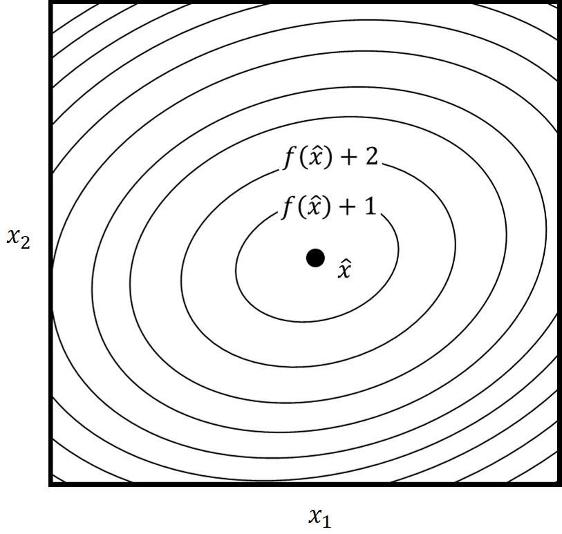
We can better understand this if we take a look at the following image.

Here we can see how the function \(\|A x-b\|^{2}=\left(2 x_{1}-1\right)^{2}+\left(-x_{1}+\right.\left.x_{2}\right)^{2}+\left(2 x_{2}+1\right)^{2} \) can be plotted as a curve. As you can see, this will give us level curves of the function. Here, the point \(\hat{x} \) minimizes he function and that will be our solution. The further away we go from the \(\hat{x} \) we will get a larger residual value. 

This already gives us a hint of how we can solve our problem. Because, if we have a convex function like this, the location of the minimum or maximum of the first derivative should be zero. 

3. How to derive the solution of the Least square problem

Now, let’s have a look at how we are going to solve the linear least-squares problem. Before we continue, we have to emphasize that there is only one condition for the data matrix \(A \) that needs to be fulfilled. That means that the columns of \(A \) are linearly independent.

So, let’s now continue with our solution. We will find the solution to the least squares problem using some basic results from calculus. If \(\hat{x} \) is minimizer of the function \(f(x)=\|A x-b\|^{2} \),  this means that we need to have the following relation satisfied:

$$ \frac{\partial f}{\partial x_{i}}(\hat{x})=0, \quad i=1, \ldots, n $$

Here, we can see that the partial derivative of \(f \) with respect to \(x_{i} \) evaluated at the value \(\hat{x} \) equals zero. Sometimes this equation is expressed as the vector equation:

$$ \nabla f(\hat{x})=0 $$

Note that here \(f \) is a function of \(\hat{x} \) where \(\hat{x} \) have \(n \) elements. Also, \(\nabla f(\hat{x}) \) is the gradient of \(f \) evaluated at \(\hat{x} \). This gradient can be expressed in the following matrix form:

$$ \nabla f(x)=2 A^{T}(A x-b) $$

This formula can be derived from the chain rule and the gradient of the sum of squares function. We can rewrite this formula as a sum of \(m \). Then if we have a sum of \(m \), we will have an \(n \) residuals. 

$$ f(x)=\|A x-b\|^{2}=\sum_{i=1}^{m}\left(\sum_{j=1}^{n} A_{i j} x_{j}-b_{i}\right)^{2} $$

To better understand this have a look at the following example:

Here, we can see the function \(f \). We have a matrix \(A \) multiplied with vector \(x \) and then the \(b \) vector is subtracted. We will multiply the first row of the matrix \(A \) with the first column of the vector \(x \), and subtract the first row of the vector \(b \). This will give us the first residual \(r_{1} \). Then we can multiply the second row of the matrix \(A \), with the second column of the vector \(x \), and subtract the second row of the vector \(b \). This will give us the value of the second residual \(r_{2} \). 

Now we need to find the partial derivative of \(f \) with respect to \(x_{j} \).

To find \(\nabla f(x)_{k} \) we take the partial derivative of \(f \) with respect to \(x_{k} \). Differentiating the sum term by term, we will get:

 $$ \nabla f(x)_{k}=\frac{\partial f}{\partial x_{k}}(x) $$

$$ =\sum_{i=1}^{m} 2\left(\sum_{j=1}^{n} A_{i j} x_{j}-b_{i}\right)\left(A_{i k}\right) $$

$$ = \sum_{i=1}^{m} 2\left(A^{T}\right)_{k i}(A x-b){i} $$

$$ = \left(2 A^{T}(A x-b)\right)_{k} $$

In our attempt to minimize this problem and find the \(\hat{x} \), we just need to solve the following equations:

$$ \nabla f(\hat{x})=2 A^{T}(A \hat{x}-b)=0 $$

This can be written as:

$$ A^{T} A \hat{x}=A^{T} b $$

These equations are called the normal equations. The coefficient matrix \(A^{T} A \) is the Gram matrix associated with \(A \). Its entries are inner products of columns of \(A \). Our initial assumption was that the columns of \(A \) are linearly independent. This implies that the Gram matrix \(A^{T} A \) is invertible. This means that we will get the following equation:

$$ \hat{x}=\left(A^{T} A\right)^{-1} A^{T} b $$

This equation is a unique solution of the normal equations that finalizes our search. 

4. Interpretation of the Least square problem

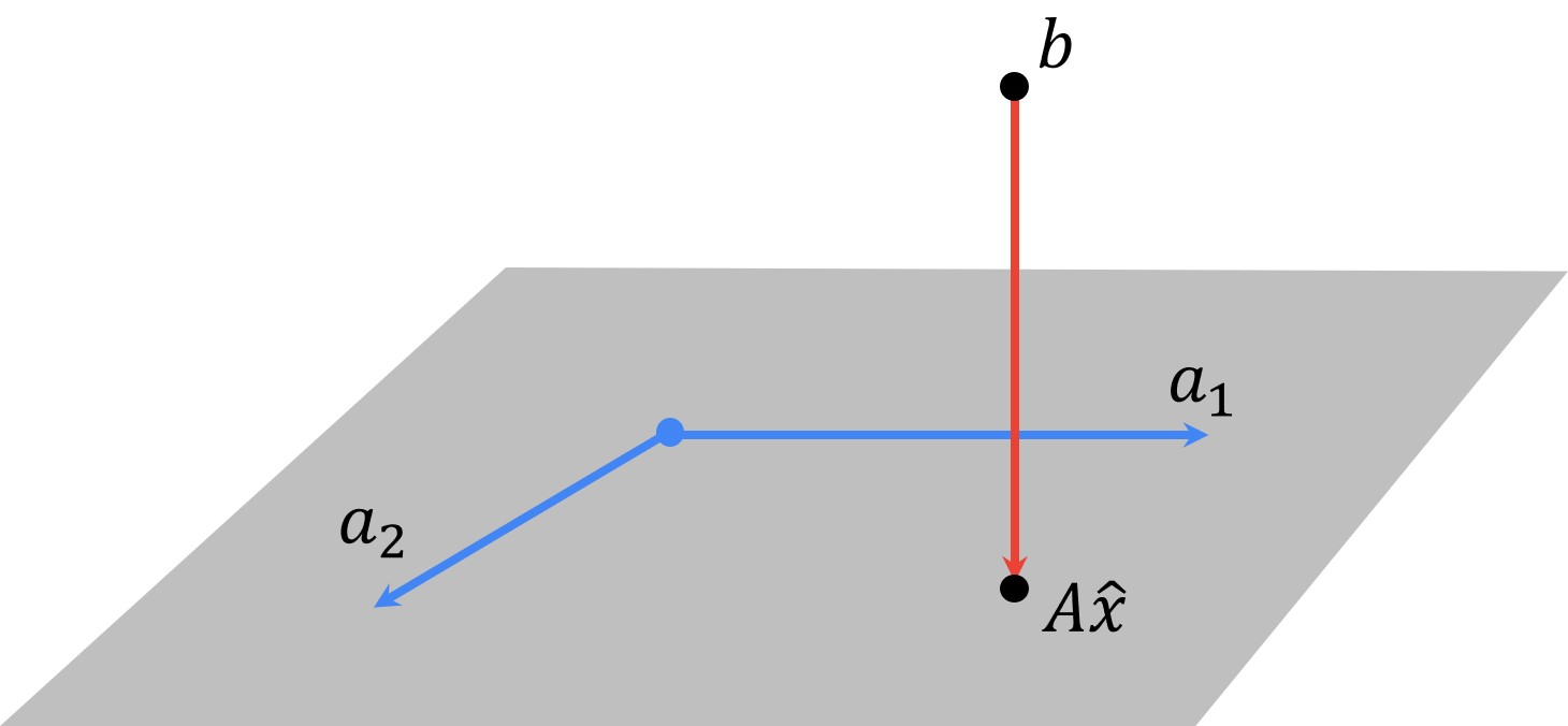
There’s an interesting interpretation of the least square problems. The point \(A \hat{x} \) is the linear combination of the columns of \(A \) that is closest to \(b \). 

So let’s say that we have a matrix \(A \) that has two columns, \(a_{1} \) and \(a_{2} \). Also, let’s assume that we have three equations. We can illustrate this example in the following way:

Because we cannot find the exact solution, \(b \) is not in this plane. This plane represents all possible vector values that we can get with combinations of vectors \(a_{1} \) and \(a_{2} \). The point \(A \hat{x} \) can be interpreted as a vector that we will get somewhere in the plane. Then, we will rotate and scale vectors, \(a_{1} \) and \(a_{2} \) within possible vector values and we will sum them. So, this can cover and span the whole plane. However, we cannot reach the point \(b \) because this point is defined in such a way that it is outside of this plane. Then this residual actually is the distance from \(b \) to this plane. If this residual \(\hat{r}=A \hat{x}-b \) is perpendicular to this plane, that will be our solution. The point \(A \hat{x} \) lies exactly where \(b \) is projected onto this plane defined by columns of a matrix \(A \), \(a_{1} \) and \(a_{2} \). The optimal residual satisfies a property that is sometimes called the orthogonality principle:

It is orthogonal to the columns of \(A \), and therefore, it is orthogonal to any linear combination of the columns of \(A \). This can be written in the following way:

$$ (A z) \perp \hat{r} $$

Here, \(z \) is any possible vector that lies in this plane and \(Az \) is always perpendicular to residual \(\hat{r} \). This concludes the least squares.

Now let’s see how we can solve the Linear least-squares problem in Python.

5. Linear least-squares example in Python

First, let’s import necessary libraries.

import numpy as npCode language: JavaScript (javascript)

Next, will create a matrix \(A \) and vector \(b \).

A = np.array ( [[2,-1,0] , [0,1,2]] ).T
ACode language: PHP (php)

array([[ 2, 0], [-1, 1], [ 0, 2]])

b = np.array ( [[1, 0 ,- 1 ]] ).T
b.shapeCode language: PHP (php)

(3, 1)

Next, we will multiply matrices \(A \) and \(A \) transposed using the command np.matmul.

C = np.matmul(A.T , A)
print(C)Code language: PHP (php)

[[ 5 -1] [-1 5]]

inv_mat = np.linalg.inv(C)
inv_mat

array([[0.20833333, 0.04166667], [0.04166667, 0.20833333]])

D = np.matmul(inv_mat , A.T) 
x = np.matmul(D, b)
print(x)Code language: PHP (php)

[[ 0.33333333] [-0.33333333]]

As you can see, our \(\hat{x}=(1 / 3,-1 / 3) \) which is the same result as in our example.

Summary

In this post, we have explained how to solve systems of linear equations that have more equations than unknowns using an algorithm called Linear least squares. To solve this problem we learned to minimize the sum of squares of errors in the equation. After deriving the solution to the Least square problem we also showed you how to solve this problem in Python.