#003 Deepfakes – Monocular 3D Face Reconstruction, Tracking, and Applications

Highlights: There has been significant progress, in the past few years, when it comes to developing techniques and algorithms for reconstructing, tracking, and analyzing human faces. The Computer Vision communities across the globe are working hard to improve the speed, accuracy, and user-friendliness of these models. As a result, many impressive case studies have presented amazing results in the most challenging problems.

Today, through this blog post, we’ll try to learn about the reconstruction and tracking of a 3-Dimensional model of a human face, using optimization-based reconstruction algorithms. So, let’s begin!

Tutorial Overview:

1. Facial Reconstruction: An Introduction
2. Input Modalities & Capture Setups
3. Image Formation Models
4. Face Models & Priors
5. Estimation Of Model Parameters
6. Applications Of Face Reconstruction
   

1. Facial Reconstruction: An Introduction

Humans have always been taken at their face values, haven’t they?

Well, faces are indeed a central part of our visual perception. They are the keys to our identities, emotions, and intents. This is the reason why researchers and computer vision communities started working on generating digital face images, in order to understand real-world faces.

This process of face capture and analysis aids Face analysis to provide useful insights into facial biometrics, face-based interfaces, visual speech recognition, and face-bashed search in visual assets. Thereby, this process helps the system in taking smart decisions.

Face analysis goes into other common applications as well, such as personalized avatar creation, 3D face printing for entertainment or medicine, and geometrical reconstruction of the face, among others. It can even aid in generating photo-realistic faces such that appearances or performances of faces can be modified within videos. Even Apple with its Face ID unlocking technology makes use of facial commodity sensors.

In this tutorial, we will understand the various optimization-based reconstruction methods which are useful in recovering and tracking a 3-dimensional model of the face. We will learn about the state-of-the-art methods currently used to make monocular reconstruction feasible, their concepts of image formation, simplifications, assumptions, and the lightweight RGB camera system they employ.

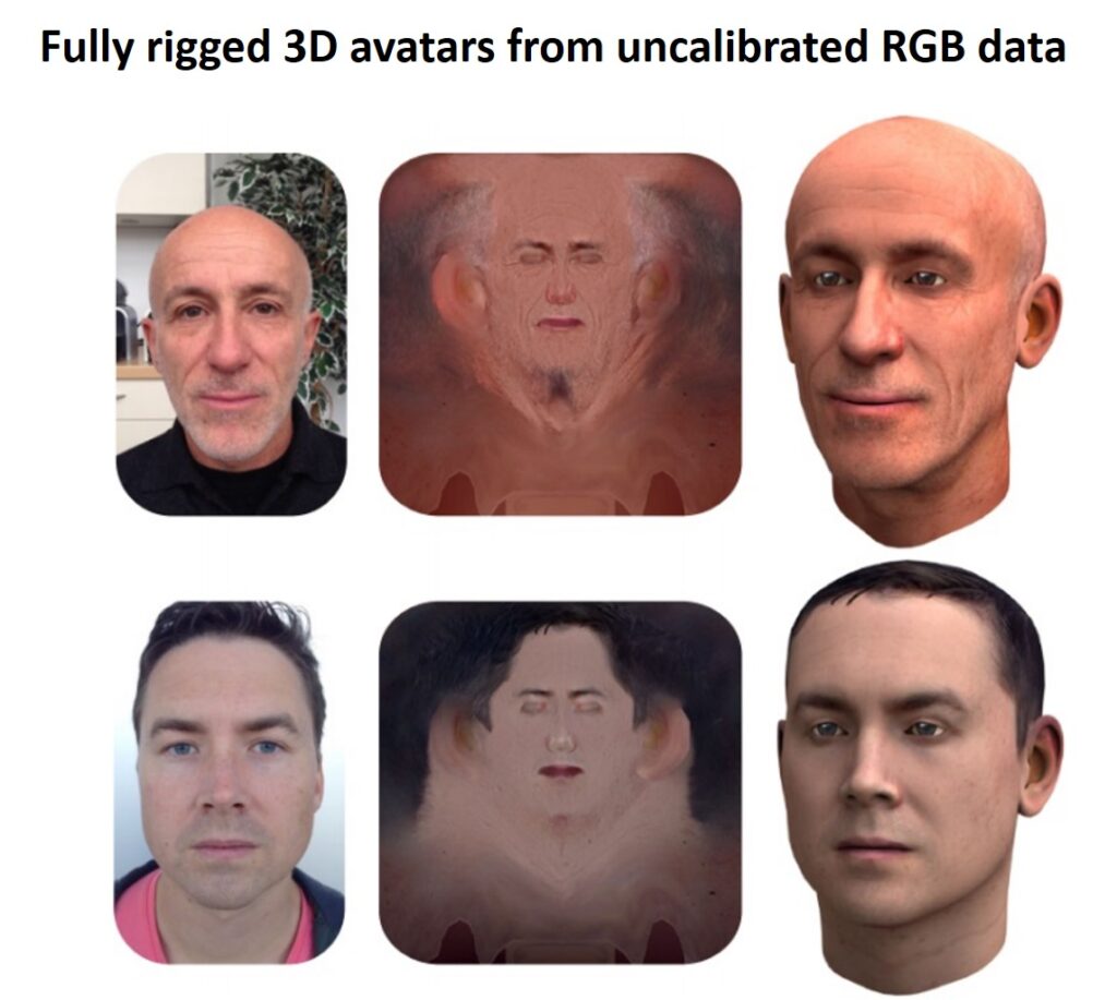
In addition, we will study the priors that allow the reconstruction of a face in the ill-posed monocular setting and how they can be acquired using high-quality capture setups. Going ahead, we will learn about the various algorithms that are modeled to extract accurate 3D deformable, textured face models from monocular RGB data, based on the described priors at off-line and real-time frame rates.

And in the end, we will understand how to use geometrical reconstructions, textures, and illuminations to accomplish complex face-editing tasks, from performance-based animation to real-time facial reenactment.

Let us begin by understanding some of the techniques used in the past and in recent times to perform face capture.

2. Input Modalities & Capture Setups

In the past, complex indoor capture setups with dense camera arrays and complex lighting setups have been used in state-of-the-art methods for facial performance capture techniques. These methods were used to reconstruct high-quality 3D face models with detailed facial motion and appearance from optical sensor measurements of a subject’s performance. However, these methods were quite expensive to build and operate.

On the contrary, the more recent methods of face capture utilize low-cost and standard monocular devices.

Let’s learn in detail about one such monocular device, known as the RGB sensor.

Monocular RGB Sensor

As the name suggests, an RGB camera captures three separate channel images that encode the amount of Red, Green, and Blue light that is being received. Such cameras are readily available, which is why these are widely used to perform monocular reconstruction and tracking methods.

Now, due to the fact that the image formation process in monocular face reconstruction and tracking convolves multiple physical dimensions in single color measurements, such as Geometry, Surface Reflectance, and Illumination, this method is highly challenging. Thus, it is considered to be an ill-posed problem.

Let us learn how the current state-of-the-art approaches employ several simplifications to achieve more effective results.

3. Image Formation Models 

Our facial geometry is mainly described using triangles or quad meshes. In most of the methods used today, the face reconstruction problem is interpreted as an inverse rendering problem. Here’s when we are required to mathematically model the entire image formation process. Many cases also involve certain material properties which describe the interaction of skin or other facial elements with the light. These need to be modeled as well.

To map from a 3D geometrical shape to a 2D image, we need to make use of projective camera models. Let us suppose we are given \(\mathbf{v} \), a 3D world point. Using this, we can obtain \(\mathbf{v} \) \(p \), a 2D image point, by following the general model as written below.

$$ \mathbf{p}=\mathbf{K} \Pi(\mathbf{R} \mathbf{v}+\mathbf{t})=\mathbf{K} \Pi(\hat{\mathbf{v}}) $$

Here, \([\mathbf{R} \mid \mathbf{t}] \in \mathbb{R}^{x+4} \) represents the camera extrinsic that transform the \(3 \mathrm{D} \) point \(\mathbf{v} \) into a point \(\hat{v} \) in camera space. \(\Pi(\cdot) \) is a non-linear operator that projects the \(3 \mathrm{D} \) point \(\hat{\mathrm{V}} \) onto the 2D image plane. And, \(\mathrm{K} \) is the geometric property of the camera. We can call these geometric properties camera intrinsics too.

Here, the projection of \(\mathbf{v} \) onto the image plane in homogeneous coordinates is represented by \(\mathbf{p}=\left[\mathbf{p}_{x}, \mathbf{p}_{y}, 1\right]^{\top} \). This point can also be represented in a non-homogenous screen space as \(\hat{\mathbf{p}}=\left[\hat{\mathbf{p}}_{x}, \hat{\mathbf{p}}_{y}\right]^{\top} \).

Moving ahead, we’ll learn how we can simplify the reconstruction of a face in the ill-posed monocular scenario. Let us understand how.

4. Face Models & Priors

In practical life, many times we are faced with incomplete and even, noisy depth data. These ill-posed monocular settings require a different set of priors wherein we model the structure and expression of a face based on low dimensional subspaces. Let’s go into detail about some of these priors.

Blendshape Expression Model

Imagine a set of 3D models of a face. While each face has a particular expression, all models have identical topologies. These 3D models are known as Blendshapes.

Interestingly, Blendshapes affect the vertex positions only. We achieve animation by blending the neutral face and a particular expression, or even by blending different expressions as shown in the image below.

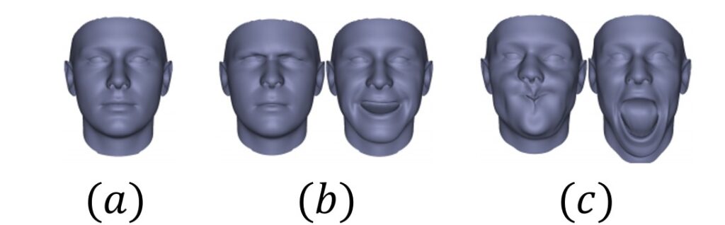
Due to their intuitive representation, Blendshapes are quite often used in 3D modeling and animation. Since each blendshape has the power to control an expression or local facial region, they are directly manipulated by artists to achieve animation. Sometimes, rather than individual blendshapes, a combination of blendshapes is used for higher-level controls.

There are two kinds of blendshape models that we are going to briefly touch upon.

1. Absolute Blendshape Model: This type of model describes the expressions of a particular face. However, it is not very commonly used as a generalized model for arbitrary faces. Have a look at the mathematical representation of this model, as written below.
   
   Suppose \(\mathbf{b}_{i}^{e} \in \mathbb{R}^{3 n} \)represents the \(m_{e}+1 \) blendshapes of a particular face, where \(\mathbf{b}_{0}^{e} \) is a neutral face. Now, we can use these blendshapes in linear combination to obtain a new facial expression \(\mathbf{e} \). This will be our absolute blendshape model.
   
   $$ \mathrm{e}=\sum_{i=0}^{m_{e}} \delta_{i} \mathrm{~b}_{i}^{e} $$
   
   Here, \(0 \leq \delta_{i} \leq 1, \forall i \in\left\{0, \ldots, m_{e}\right\} \) represent the blendshape weights. The parameter limits are under the assumption that each individual blendshape models the maximal allowed activation of the corresponding expression.
   
2. Delta Blendshape Model: While the Absolute Blendshape Model can only describe animations of one particular face, Delta Blendshape Model can be used to generalize for all kinds of faces. This is much more convenient and popularly used by modeling packages such as Maya. Let us understand this model mathematically.
   
   Well, in the case of Delta Blendshape Model, the equation for obtaining the neutral face, \(\mathbf{b}_{0}^{e} \), becomes:
   
   $$ \mathbf{e}=\mathbf{b}_{0}^{e}+\sum_{i=1}^{m_{e}} \delta_{i}\left(\mathbf{b}_{i}^{e}-\mathbf{b}_{0}^{e}\right)=\mathbf{b}_{0}^{e}+\sum_{i=1}^{m_{e}} \delta_{i} \mathbf{d}_{i}^{e} $$
   
   Here, \(0 \leq \delta_{i} \leq 1 \) and \(\mathbf{d}_{i}^{e}, \forall i \in\left\{1, \ldots, m_{e}\right\} \) are the per-vertex 3D displacements w. r. t. the neutral face \(\mathbf{b}_{0}^{e} \) .
   
   We can combine this Delta Blendshape Model with another model (Parametric Face Model) that we will study ahead to obtain a general face model equation with shape and expression.
   
   $$ \mathbf{s}=\mathbf{a}_{s}+\sum_{i=1}^{m_{s}} \alpha_{i} \mathbf{b}_{i}^{s}+\sum_{i=1}^{m_{e}} \delta_{i} \mathbf{d}_{i}^{e} $$
   
   To understand the above expression fully, let us talk about the other model we included above, known as the Parametric Face Model.
   

Parametric Face Model

The Parametric Face Model has been proposed by Blanz and Vetter. This commonly-used model is constructed using a database of 200 human faces with a neutral expressions. These expressions were digitized using a laser scanner. Therefore, we can say that all the faces used in this model have the same topology. But, they differ in geometry and skin reflectance.

The template mesh is a simple triangle mesh that consists of \(n \) vertices. Principal Component Analysis (PCA) is applied to geometry and skin reflectance, independently. This reduces the dimensionality of the dataset by a great deal. It also helps in computing the principal components of the dataset along with the corresponding standard deviations. These deviations are based on the assumption of a multivariate Gaussian distribution of samples. Let us understand this mathematically.

Let the\(\mathbf{b}_{i}^{s} \in \mathbb{R}^{3 n} \) and \(\mathbf{b}_{i}^{r} \in \mathbb{R}^{3 n} \) be the \(m_{s} \) shape and \(m_{r} \) reflectance basis vectors, respectively. The vectors \(\mathbf{b}_{i}^{S} \) contain the stacked \(x \), \(y \), \(z \) components of all vertices and \(\mathbf{b}_{i}^{r} \) the \(r, g, b \) -components respectively.

Now, the PCA model is used to synthesize new faces (shape \(\mathbf{s} \) and skin reflectance \(\mathbf{r} \)) through linear combination, as represented below.

$$ \mathbf{s}=\mathbf{a}_{s}+\sum_{i=1}^{m_{s}} \alpha_{i} \mathbf{b}_{i}^{s} $$

$$ \mathbf{r}=\mathbf{a}_{r}+\sum_{i=1}^{m_{r}} \beta_{i} \mathbf{b}_{i}^{r} $$

In the above expressions, the average face is represented by \(\mathbf{a}_{s} \in \mathbb{R}^{3 n} \) and the average reflectance is denoted by \(\mathbf{a}_{r} \in \mathbb{R}^{3 n} \) New shapes \(\mathbf{s} \) and reflectances \(\mathbf{r} \) are generated by adding a linear combination of the basis vectors \(\mathbf{b}_{i}^{s} \) and \(\mathbf{b}_{i}^{r} \) using weights \(\alpha_{i}\) and \(\beta_{i} \), respectively. The corresponding standard deviations \(\sigma_{s} \in \mathbb{R}^{m_{s}} \) and \(\sigma_{r} \in \mathbb{R}^{m_{r}} \) are stored in vectorized form.

While both the models, Blendshape for expressions and Parametric for shapes, are effective in regularizing the ill-posed reconstruction problem and enabling high-quality results, they are still restrictive when it comes to fine-scale skin detailing such as wrinkles.

Advanced Face Models

Let us look at some pictorial examples of advanced face models involving Fine-Scale Detail Estimation and Reconstruction of Personalized Face Rigs.

The facial performance capture approach of Garrido et al. makes use of shape-from-shading techniques to reconstruct wrinkle-level surface detail.

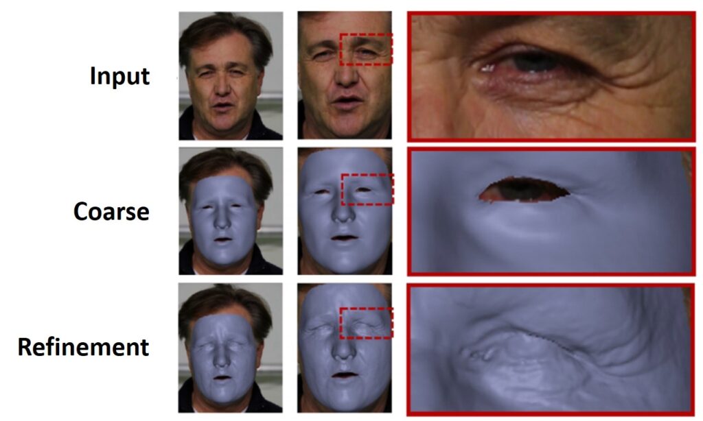
The real-time high-fidelity facial performance capture by Cao et al. employs the RGB input to compute a texture map based on the coarse mesh. This allows the regression of wrinkle-level detail at real-time frame rates based on commodity data.

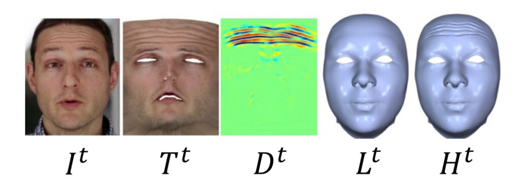
And, finally, the dynamic 3D avatar creation from hand-held video input by Ichim et al. is based on learning a linear mapping between fine-scale details and facial feature strain. Using this, adding wrinkles to the synthesized expressions becomes easy. Have a look.

Now that we have learned about the different face models and priors, let us understand how to estimate and optimize the parameters of a particular face model.

5. Estimation of Model Parameters 

In all, there are two approaches for estimating the parameters of a face model – generative and discriminative. The generative approach utilizes the principle of analysis-by-synthesis based on parameter optimization. This involves minimizing the difference between the synthetic image and the observed image in an iterative manner. We call this ‘Energy Minimization’. Other than parameter optimization, the generative approach can also be based on parameter regression.

To start with, let’s understand Energy Minimization based on parameter optimization.

Energy Minimization

Say, we are given an input which is a monocular video. In this scenario, we estimate our parameters by considering them as a general non-linear optimization problem.

Mathematically speaking, we’ll optimise the following parameters: Global head rotation \(\mathbf{R} \) and translation \(\mathbf{t} \), facial shape \(\left\{\alpha_{i}\right\}_{i=1}^{m_{s}} \), reflectance \(\left\{\beta_{i}\right\}_{i=1}^{m_{r}} \), expression \(\left\{\delta_{i}\right\}_{i=1}^{m_{e}} \) and illumination \(\left\{l_{i}\right\}_{i=1}^{m_{l}} \)

Now, in order to find the optimal parameters \(\mathcal{P}^{*} \), we must minimize a reconstruction/tracking objective function \(E \), as shown below.

$$ \mathcal{P}^{*}=\underset{\mathcal{P}}{{argmin}} E(\mathcal{P}) $$

The used tracking objectives in the unknown parameters are highly non-linear and generally, include these components:

$$ E(\mathcal{P})=\underbrace{w_{\text {dense }} E_{\text {dense }}(\mathcal{P})+w_{\text {sparse }} E_{\text {sparse }}(\mathcal{P})}_{\text {data }}+\underbrace{w_{\text {reg }} E_{\text {reg }}(\mathcal{P})}_{\text {prior }} $$

As you can see, the above components are essentially in two parts – the data and the prior. The data components measure the similarity of the current synthesized face and the input data. Among these data terms, the Sparse feature alignment terms, \(E_{\text {sparse }} \), match a small number of feature points of the model to equivalent detected feature points in the input. You can check out the influence of different alignment terms, also known as the Energy terms, in the image below.

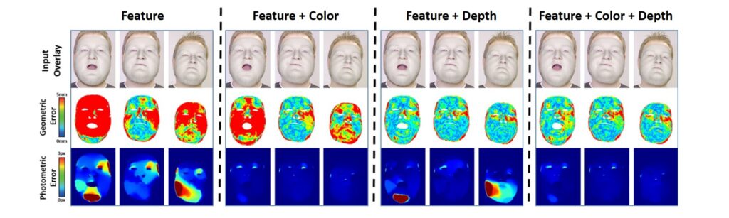
The image above shows that we can see how tracking accuracy is computed in terms of geometric and photometric error. This results in a final reconstructed pose, which is an overlay on top of the input images.

In the example above, the mean and standard deviations of geometric and photometric error are \(6.48mm/4.00mm \) and \(0.73px/0.23px \) for Feature, \(3.26mm/1.16mm \) and \(0.12px/0.03px \) for Features+Color, \(2.08mm/0.16mm \) and \(0.33px/0.19px \) for Feature+Depth, \(2.26mm/0.27mm \) and \(0.13px/0.03px \) for Feature+Color+Depth.

Now, let us look at the terms or components of our Energy Minimization equation in detail.

1. Sparse Feature Alignment: This is one of the most important data terms in Energy Minimization when it comes to dealing with the many visually salient features of faces.
   
   $$ E_{\mathrm{lan}}(\mathcal{P})=\frac{1}{|\mathcal{F}|} \sum_{\mathbf{f}_{j} \in \mathcal{F}} w_{\mathrm{conf}, j}\left\|\mathbf{f}_{j}-\mathbf{K} \Pi\left(\mathbf{R} \cdot \mathbf{v}_{j}(\mathcal{P})+\mathbf{t}\right)\right\|_{2}^{2} $$
   
   It enforces that a small set of facial landmark points \(\mathbf{v}_{j}(\mathcal{P}) \) on the model align well with corresponding detected 2D features \(\mathbf{f}_{j} \in \mathcal{F} \subset \mathbb{R}^{2} \). Each of the detections normally comes with a confidence \(w_{\text {conf }, j} \) that can be used to weight the corresponding alignment constraint.
   
   Many methods exist for detecting and tracking facial features and landmarks, some of which are holistic and use the entire facial region to localize landmarks. One such holistic method is the Active Appearance Model (AAM).
   
   Now, as we know that the Energy Minimization problem is highly non-linear, which makes \(E_{\text {lan }} \) a very important energy term. If it weren’t for this data term, we won’t be able to track fast motion and strong deformation reliably. The facial feature points in this data term initialize the tracker in the first frame along with bringing the optimization close to the basin of convergence of the dense alignment constraints.
   
2. Dense Photometric Alignment: Unlike Sparse Feature Alignment, Dense Photometric Alignment measures how well the input data is explained by a rendered version of the current fit:
   
   $$ E_{\mathrm{col}}(\mathcal{P})=\frac{1}{|\mathcal{V}|} \sum_{\mathbf{p} \in \mathcal{V}}\left\|C_{\mathcal{S}}(\mathcal{P}, \mathbf{p})-C_{\mathcal{I}}(\mathbf{p})\right\|_{2}^{2} $$
   
   Here, the synthesized face image is represented by \(C_{\mathcal{S}} \), the input RGB image is represented by \(C_{\mathcal{I}} \) and the visible pixel positions in \(C_{\mathcal{S}} \), used for comparison, are denoted by \(\mathbf{p} \in \mathcal{V} \).
   
3. Dense Geometric Alignment: This data term makes use of the available depth stream and constraints the reconstruction problem in a better way, thereby, resolving the depth ambiguity. All RGB-D-based approaches rely on this data term, apart from the dense photometric constraints.
   
   A sum of the projective Euclidean point-to-point distances to the input is an effective constraint to measure the point-to-point distance between model surface points and input depth. This ensures that the reconstructed geometry of the face model is tightly aligned to the captured depth stream.
   
   Here’s how we represent this constraint mathematically:
   
   $$ E_{\mathrm{point}}(\mathcal{P})=\frac{1}{|\mathcal{V}|} \sum_{\mathbf{p} \in \mathcal{V}}\left\|X_{\mathcal{S}}(\mathcal{P}, \mathbf{p})-X_{\mathcal{I}}(\mathbf{p})\right\|_{2}^{2} $$
   
   Here, \(X_{\mathcal{S}}(\mathcal{P}, \mathbf{p})-X_{\mathcal{I}}(\mathbf{p}) \) is the difference between the measured 3D position and the corresponding 3D model. \(\mathcal{V} \) signifies all the visible pixel positions that are used for comparison. Many times, this constraint is defined on a vertex level rather than a pixel level.
   
   In order to improve the robustness and convergence of this constraint, we often use a first-order surface approximation, that benefits translational motion. Here is how we use it.
   
   $$ E_{\text {plane }}(\mathcal{P})=\frac{1}{|\mathcal{V}|} \sum_{\mathbf{p} \in \mathcal{V}}\left[N_{\mathcal{S}}(\mathcal{P}, \mathbf{p})^{\top} \cdot\left(X_{\mathcal{S}}(\mathcal{P}, \mathbf{p})-X_{\mathcal{I}}(\mathbf{p})\right)\right]^{2} $$
   
   Here, \(N_{\mathcal{S}} \) represents the synthesized surface normal image.
   
4. Regularization: This term is used to further constrain the reconstruction problem and resolve ambiguities. Mathematically, we can represent this constraint in the following way.
   
   $$ E_{\mathrm{reg}}(\mathcal{P})=\sum_{i=1}^{m_{s}}\left(\frac{\alpha_{i}}{\sigma_{s, i}}\right)^{2}+\sum_{i=1}^{m_{r}}\left(\frac{\beta_{i}}{\sigma_{r, i}}\right)^{2}+\sum_{i=1}^{m_{e}}\left(\frac{\delta_{i}}{\bar{\sigma}_{e, i}}\right)^{2} $$
   
   Regularization is often used to prevent degeneration of the facial geometry and face reflectance.

So, this was about Energy Minimization. Let us move ahead and talk about Model Initialization.

Model Initialization 

Often, the approaches we are using employ multiple images right at the beginning of the input sequence. This is, in fact, better because this helps us estimate the identity more efficiently than reconstruction from a single frame.

For example, the strategy proposed by Weise et al. fuses multiple depth frames based on rigid alignment, to obtain a 3D model of the neutral face. Even Thies et al. proposes a strategy that utilizes model-based non-rigid bundle adjustment. This is done with different head poses, over 3 frames. In addition, the strategy by Ichim et al. involves performing a static structure-from-motion reconstruction. This approach averages the identity over a small part of a particular video and is based on the multi-view data captured by an iPhone.

Now, let us look at another important aspect of the analysis-by-synthesis approach for estimation of parameters, i.e., the Optimisation problem.

Optimization Strategies

As we learned earlier, the analysis-by-synthesis approach involves the estimation of face parameters. These parameters minimize the difference between the synthesized image and the input image of a face.

This kind of approach computes a new set of parameters \(\mathcal{P}^{i+1} \) iteratively, taking the synthesis generated with the old parameters, \(\mathcal{P}^{i} \), as the starting point. To minimize the energy that measures the difference between the synthetic image and the observed image, the parameters \(\mathcal{P}^{i+1} \)are taken into consideration.

Suppose we have an objective function \(E(\mathcal{P}) \) that consists of a single data fitting term represented by the following expression.

$$ E(\mathcal{P})=\frac{1}{|\mathcal{V}|} \sum_{\mathbf{p} \in \mathcal{V}} \Psi(\mathbf{r}(\mathcal{P}, \mathbf{p})) $$

In the expression above, \(\Psi: \mathbb{R}^{n} \rightarrow \mathbb{R}_{\geq 0} \) is a function that maps the difference \(\mathbf{r}(\mathcal{P},\mathbf{p})=C_{\mathcal{S}}(\mathcal{P},\mathbf{p})-C_{\mathcal{I}}(\mathbf{p}) \) between the observations and the model to a scalar. The number of residuals often changes with iterations and is proportional to the number of pixels or the number of vertices.

Now, let’s see how we can transform our optimization problem into a nonlinear least squares problem. Employing a commonly used metric \(\ell_{2}\) -norm \(\left(\Psi(\mathbf{x})=\|\mathbf{x}\|_{2}^{2}\right) \), we can rewrite the above expression as follows.

$$ E(\mathcal{P})=\frac{1}{|\mathcal{V}|} \sum_{\mathbf{p} \in \mathcal{V}}\|\mathbf{r}(\mathcal{P}, \mathbf{p})\|_{2}^{2}=\|F(\mathcal{P})\|_{2}^{2} $$

Interestingly, if \(F(\mathcal{P}) \) is a linear function in the model parameters \(\mathcal{P} \) the optimization problem becomes a much simpler linear least squares problem \(\left(\|\mathbf{A} \mathcal{P}+\mathbf{b}\|^{2} \rightarrow \min \right) \). Now, this can easily be solved using the corresponding normal equations \(\mathbf{A}^{\top} \mathbf{A} \mathcal{P}=-\mathbf{A}^{\top} \mathbf{b} \).

However, in most of the existing state-of-the-art approaches,\(F(\mathcal{P})\) is a nonlinear function. This is because of the perspective camera assumption. For solving this system of nonlinear equations using the least-squares problem, we make use of iterative methods such as the Gradient Descent Method, the Gauss-Newton Method, and the Levenberg-Marquardt Method. You can read up about these methods in detail, in our previous tutorial about Nonlinear Equations.

Now, let’s calculate the general solution for our nonlinear problem using Newton’s method.

$$ \mathcal{P}^{i+1}=\mathcal{P}^{i}-\mathbf{H}_{E}\left(\mathcal{P}^{i}\right)^{-1} \cdot \nabla E\left(\mathcal{P}^{i}\right) $$

Here, \(\nabla E\left(\mathcal{P}^{i}\right) \) represents the gradient and \(\mathbf{H}_{E}(\mathcal{P}) \) denotes the Hessian of the energy function. This involves the second order derivatives of the residual vector \(F(\mathcal{P}) \) as well.

Note that the Gauss-Newton method is only restricted to nonlinear least-squares problems and approximates the Hessian using only first-order derivatives, as shown below.

$$ \mathbf{H}_{E}(\mathcal{P}) \approx 2 \cdot \mathbf{J}^{\top}(\mathcal{P}) \cdot \mathbf{J}(\mathcal{P}) $$

In the expression above, \(\mathbf{J}(\mathcal{P}) \) signifies the Jacobian of the residual function \(F(\mathcal{P}) \). We can use this approximation and derive the following expression.

$$ \mathcal{P}^{i+1}=\mathcal{P}^{i}-\underbrace{\left[\mathbf{J}^{\top}\left(\mathcal{P}^{i}\right) \cdot \mathbf{J}\left(\mathcal{P}^{i}\right)\right]^{-1} \cdot \mathbf{J}^{\top}\left(\mathcal{P}^{i}\right) \cdot F\left(\mathcal{P}^{i}\right)}_{\Delta^{i}} $$

And thus, in order to calculate the parameter update \(\Delta^{i} \), we must solve the following system of linear equations.

$$ \left[\mathbf{J}^{\top}\left(\mathcal{P}^{i}\right) \cdot \mathbf{J}\left(\mathcal{P}^{i}\right)\right] \cdot \Delta^{i}=\mathbf{J}^{\top}\left(\mathcal{P}^{i}\right) \cdot F\left(\mathcal{P}^{i}\right) $$

Apart from the above metric, we have another common metric that uses the Iteratively Reweighted Least Squares (IRLS) method. We can write this metric as \(\ell_{2,1} \) -norm \(\left(\Psi(\mathbf{x})=|\mathbf{x}|_{2}^{1}\right) \).

The IRLS method transforms our optimization problem into a sequence of nonlinear least-squares problems by splitting the norm into two key components: Constant and Least Squares (optimized by the Gauss-Newton method as shown above). Have a look.

$$ \|\mathbf{r}(\mathcal{P}, \mathbf{p})\|_{2}^{1}=\underbrace{\left(\|\mathbf{r}(\mathcal{P}, \mathbf{p})\|_{2}^{1}\right)^{-1}}_{\text {constant }} \cdot \underbrace{\|\mathbf{r}(\mathcal{P}, \mathbf{p})\|_{2}^{2}}_{\text {least-squares }} $$

While optimization is an important step, it is still computationally expensive. There have been researches and proposals of newer approaches that could bypass the costly optimization process. Let us understand these new approaches better.

Machine Learning For Dense Face Reconstruction

In order to eliminate the optimization step, a recent approach has been proposed, which involves a regression function that directly estimates the model parameters from a given video sequence.

Regression of a small number of control points is often used to fit a parametric face model. However, now, even machine learning-based approaches can effectively perform dense face reconstruction.

While some of the other approaches involve monocular face reconstruction from a single input image, these new approaches utilize Random Forests and even Deep Convolutional Networks (CNNs). This helps in learning the image-to-parameter or image-to-geometry mapping directly from a training corpus.

These were some of the ways and approaches for estimating parameters in face reconstruction models, either generatively or discriminatively.

Face reconstruction is such a fascinating and revolutionary subject that it finds application in many new-age problems and has the capability to enable many technological innovations. Let’s see how.

6. Applications Of Face Reconstruction

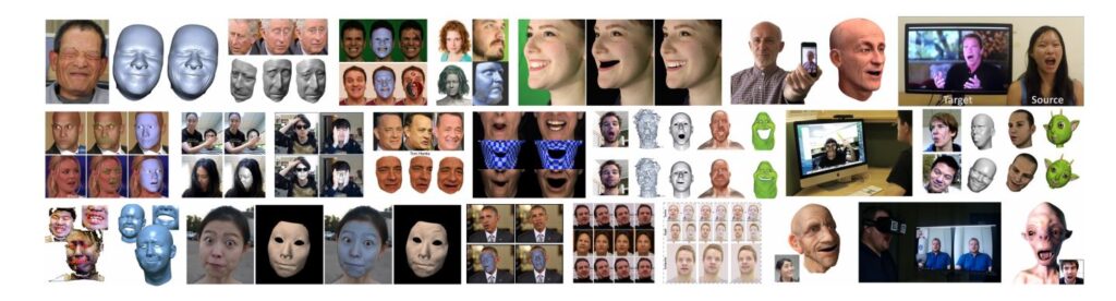
Many exciting applications make use of dense face reconstruction and tracking due to their lightweight capture setups. Let’s discuss some of these applications briefly.

Facial Puppetry

Everybody loves creating and tinkering with digital avatars. How are these digital avatars animated? Well, the answer lies in Facial Puppetry.

Facial Puppetry is basically cloning and transferring of expressions and emotions of a user from an input video stream to a target character rig. This video-driven facial animation is quite often utilized in the movie and game industry.

There are essentially two ways of meaningful facial expression cloning.

1. Parameter-based methods, which directly transfer parameters between the source and the target.
2. Motion-based methods, which map the dense 2D facial motion of the source video onto the 3D geometry of the target rig.

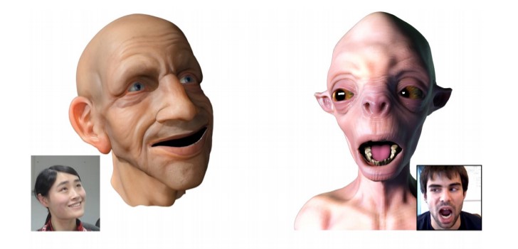
Above is a pictorial representation of a Facial Puppetry system, demonstrated by Cao et al. and Bouaziz et al., in real-time.

Face Replacement

Another great application of face reconstruction involves the swapping of faces. Imagine replacing an actor’s from a video with the face of a source actor, wherein the two videos are recorded under completely different illumination conditions.

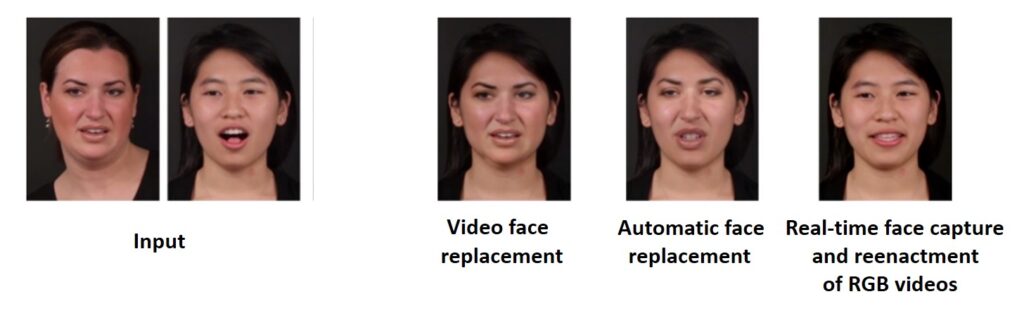
Face Replacement technology synthesizes a novel sequence that looks realistic and maintains temporal consistency, such that the target face identity remains intact and only the expressions are adapted accordingly. This process can also be seen in the example above.

Facial Reenactment

Face reconstruction is also used in facial reenactment, which involves transferring facial expressions from a source actor to a target actor’s original video face content. This is done using normalized motion fields, space-time transfer, motion parameters, or simulating motion via image-based interpolation of candidate frames. These frames are selected either manually or using a similarity metric.

A special case of facial reenactment is when the source actor and the target actor are the same people. This is known as Self-Reenactment.

Have a look at this example.

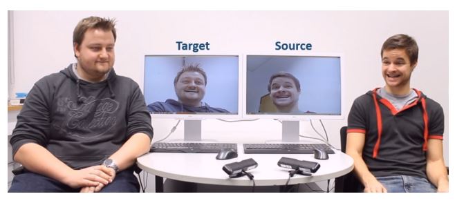
In the example image above, we can see the source actor on the right is driving the target LIVE video on the left. The device that was used to capture both the actors is the Asus Xtion Pro depth camera.

Another example of Face Reenactment can be seen below, which demonstrates the Face2Face approach that synthesizes the mouth interior using actual mouth frames from the target video.

As we can see above, the Face2Face approach reconstructs the geometry and skin reflectance of a person based on monocular RGB input. This makes it a good application for the facial reenactment of internet videos.

Speech-Driven Animation

Not just video-to-video, but even sound-to-video reconstruction is possible with Speech-Driven Animation. Herein, Phonemes (the units of sound) are associated with Visemes (the units of visual) to synthesize new mouth animations. These Phonemes are extracted from audio streams or even texts (using advanced speech processing techniques) and are mapped using boundary mismatch constraints to their counterpart Visemes.

Video Dubbing

The key idea behind Video Dubbing is to transform the motion of the mouth such that it aligns with the mouth of a dubbing actor who is speaking a foreign language. It can be said that Video Dubbing is an extension or a form of Face Reenactment, wherein facial deformations are only transferred in the mouth region.

An interesting application of Video Dubbing technology is in LIVE multilingual teleconferences where an interpreter translates a person’s speech simultaneously while she/he speaks.

Virtual Make-Up

Wouldn’t it be wonderful to have a virtual mirror that tells you that you are beautiful every time?

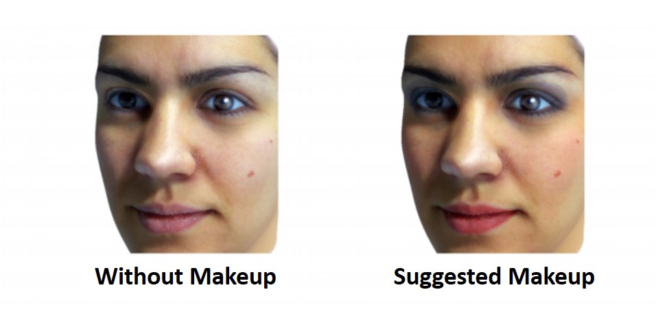
Virtual Make-Up enables users to change the texture of the reconstructed face. This means that the new face can have tattoos, logos, or modified illumination, depending on the reconstruction algorithm, as shown in the example image below.

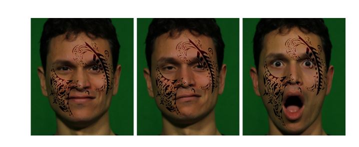
Based on a learned mapping between observations with bare skin and make-up, the process of facial make-up as suggested by Scherbaun et al. is also a popular application with photo-realistic results.

The research on the subject of Face Reconstruction is cutting-edge indeed and we sincerely hope it will continue to expand into many more innovative applications.

That’s it for this post! We hope it was interesting for you to learn about a topic that’s so relevant in today’s lifestyle. Performance-based facial animation, video manipulation, and real-time facial reenactment are surely the next big things in the digital world of the future. Before, we go, let’s summarise everything that we learned today.

Monocular 3D Face Reconstruction, Tracking and Applications

• Face analysis is an important parameter for decision-making when it comes to identity and emotions
• Multi-view capture setups can help reduce dimensionality and aid in real-world image formation
• 3D geometry is mapped to 2D images using projective camera models
• Statistical priors are used to reconstruct faces in ill-posed monocular settings or in the case of noisy and incomplete depth data
• Simpler face models give high-quality results for the ill-posed reconstruction problem but lack fine-scale skin detail and person-specific idiosyncracies
• Estimation of model parameters is done either by using analysis-by-synthesis or Energy Minimization or by using regression techniques involving Deep CNNs
• Face reconstruction has many applications such as Face Cloning, Face Replacement, Face Reenactment, Video Dubbing, and Virtual Make-ups
  

Summary

This particular blog post, in particular, is one of my favorites ever! The sheer potential of 3D Face Reconstruction is so immense that it can alter the reality of our future. We may think we are already in the digital era but we have no idea what is in store for us tomorrow. A game-changing deep digital explosion is soon to begin. Are you ready to dive into it? If not, maybe your avatar might be more willing. We’ll see you soon in our next post. Take care! 🙂