#006 3D Face Modeling – A Morphable Model for the synthesis of 3D Faces

Highlights: Hello and welcome. In this post, we shall describe a modeling technique for 3D textured faces. By converting a set of 3D face models’ shapes and textures into a vector space representation, we will be able to create a morphable face model. By creating linear combinations of face models, new faces and facial expressions can be generated. So, let us begin this journey!

3D Database of Faces (Cyberware TM)

In order to create 3D models of faces, first we need to train a model. For that, we need to create a database. The databases that are used for this kind of research are 3D scans of peoples’ heads. In this paragraph, we will explore how such a dataset is obtained.

Initially, the heads of 200 young people were scanned. From this number, 100 were male and 100 were female. The output of this scanner was a head data structure in a cylindrical representation. This provides coordinates \(r(h, \phi) \) that tell us how faces are sampled. The \(h \) angle is the horizontal spacing, where the vertices are located in the x direction, and the \(\phi\) in the y, or vertical direction. Additionally to these angles, we get RGB colors of the points on the face.

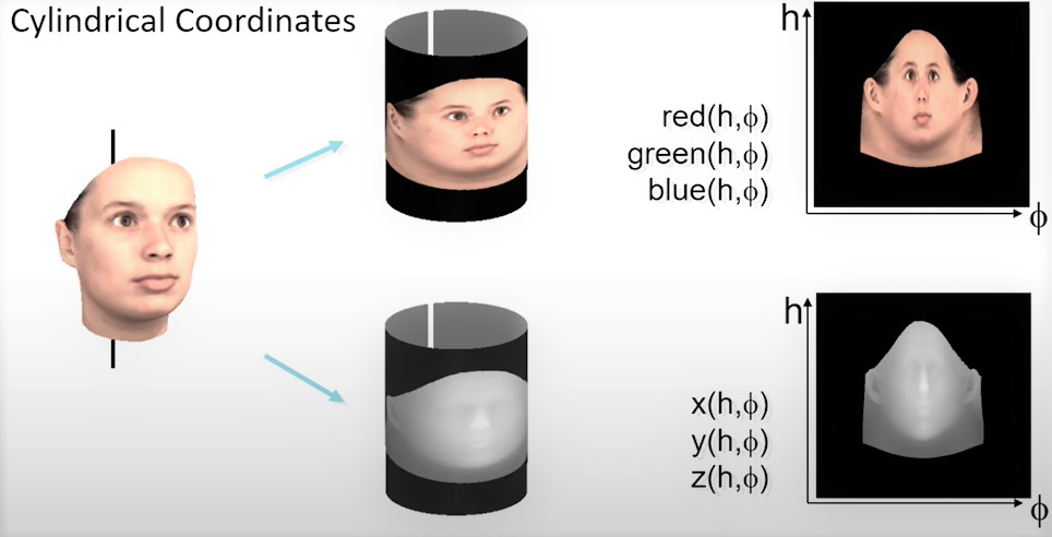
This scanner in the end gives us 70,000 vertices (3D coordinates) and the same number of color values, the color of each pixel in those vertices. This is shown in following figure 1.

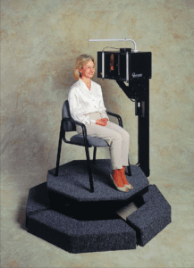
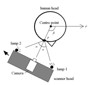
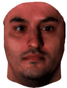
Below you can find several images showcasing the device, and what the face scans look like. Also, you can see some results [1].

Introduction to Morphable Face Models

Using the database above, the researchers at Max Planck Institute for Biological Intelligence created a morphable face model, Volker Blanz and Thomas Vetter 1999. However, they didn’t just want to create a static model. Instead, they wanted a model that can be used in later research to generate new faces just from 2D input (images). In this way, they wouldn’t need the scanner anymore, just pictures.

Let us now explore this process in a little bit more detail now.

A 2D input image is taken and placed in something the researchers call Face Analyzer. The goal of this analyzer is to return a 3D mesh of the face. Interestingly, if we were to take this 3D mesh and project it back onto the image plane it should create the same or a very similar image as the one that we started with.

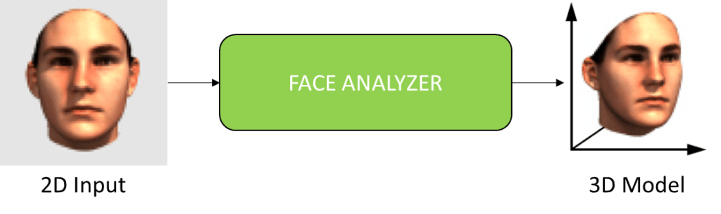
However, it is not just important to create this 3D model and project it into 2D space. We want to be able to control facial movements, expressions, and other facial features. In a 3D model, there are coefficients that can be modified and when modified they perform different modifications on the 3D model. Some of these coefficients can perform rigid transformations (rotation and translation), and some non-rigid transformations (shape, expressions, etc.). The idea is that if we take the 3D face model and modify some coefficients, we can create different variations of the face and when this 3D face is projected into 2D we obtain new images. This method was presented in one of the most influential papers [2] on how a 3D face can be obtained.

Morphable 3D Face Model

As we already discussed, morphable face models are created using a database of 3D face scans. For each face, we will have a shape vector \(S=(X_1, Y_1, Z_1, X_2, Y_2, Z_2, …, X_n, Y_n, Z_n)^T \in \mathbb{R}^{3n}\) which contains \(X, Y, Z\) coordinates of each of the \(n\) vertices. However, in addition to the coordinates, we also obtain the RGB values for each of the coordinates (shown in Figure 1). After obtaining all of these vectors, assuming that all the faces are aligned, a new shape \(S_{model}\) and new texture \(T_{model}\) is created as a linear combination of the shapes and textures of the \(m\) faces.

$$ S_{model} = \sum^{m}_{i=1} a_i S_i \quad \textrm{,} \quad T_{model} = \sum^{m}_{i=1} b_i T_i \quad \textrm{,} \quad \sum^{m}_{i=1} a_i = \sum^{m}_{i=1} b_i = 1 $$

To visualize this, let us look at figure 6 which is shown below. For example, by linearly combining all the green 3D vectors we can create a new vector in this 3D space (the red vector).

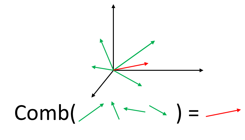
So, in this paper, authors assume that for a large number of faces they will be correlated. We can perform linear combinations over different faces and obtain new faces (imagine the vectors in Figure 6 as faces). Also, all the colors can be reconstructed as a linear combination as well. But, this dataset consists dominantly of Caucasians and some other people may not be able to reconstruct their faces.

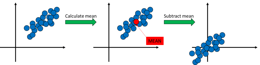
The next step would be to fit a multivariate normal distribution on the data. This is done based on the averages of shapes \(\bar{S}\) and textures \(\bar{T}\) and the covariance matrices \(C_S\) and \(C_T\). Let’s explore this in a little bit more detail.

After finding the mean of the shapes and textures, we want to obtain the covariance matrices. For this, we need to subtract the mean values from the data points. What does this do in practice? In practice, this means that the points are shifted in a way that the origin is in the middle of the points, Figure 7.

After the data points have been shifted, or zero-meaned as researchers call it, the next step is to calculate the covariance matrices \(C_S\) and \(C_T\) over the shape and texture differences.

$$ \triangle S_i = S_i – \bar{S} \quad \textrm{and} \quad \triangle T_i = T_i – \bar{T} $$

What does the covariance matrix show us? It shows us the variance and covariance in the dataset. The diagonal elements of the matrix represent the variance (how much is the data spread) and the covariance can be positive/negative/zero representing the relationship between features in the dataset (zero means that two features do not vary together).

Once we compute these covariance matrices, we perform PCA which will help us in finding eigenvectors and eigenvalues. If you need to refresh your knowledge of PCA read this post.

By applying PCA we will get principal components that will tell us how big of an impact they have and which can be ignored. This way we will be able to achieve similar results as by using all the components. The researchers in this paper [2] found that only 80 principal components are enough to preserve the final results. Looking at the formula below, we can see two new variables \(\alpha\) and \(\beta\), which indicate a weight. This weight is assigned next to each coefficient, and if a coefficient is having a big impact on the overall result, this weight will be larger.

$$ S_{model} = \bar{S} + \sum_{i=1}^{m-1}\alpha_is_i \quad \textrm{,} \quad T_{model} = \bar{T} + \sum_{i=1}^{m-1}\beta_it_i $$

Segmented Morphable Models

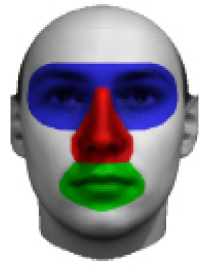
The scientists also introduced a segmented morphable model, which is the idea of modeling independent parts of the face separately. It is presented as a nice idea, but in our case, we will use a holistic unified approach to treat our model without segmentation. For example, modeling of the eyes, nose, mouth, and other regions (Figure 8).

Facial Attributes

The shape and texture coefficients, \(\alpha\) and \(\beta\), that are used in the Morphable Face Model for PCA representation do not correspond to facial attributes as we humans would describe them. For instance, they are referring to facial femininity, being bony, and so on. This is challenging to be described and captured in numbers, but what scientists do, is define one method of how this still would be possible. They want to find which of these vertices are dominant for which corresponding facial attribute.

So, how can we do this? By capturing two scans of the same person but with different emotions. For example, one person is in a neutral state, and the same person is smiling. We take these two scans and subtract them.

$$ \triangle S = S_{expression} – S_{neutral} \quad \textrm{,} \quad \triangle T = T_{expression} – T_{neutral} $$

In this way, \(\triangle S\) and \(\triangle T\), vertices that are showing large absolute values are the ones where was a difference. This way we can detect which are used for a smile, for this example the lip region.

However, unlike facial expressions, there are attributes that are subject invariant, meaning that they are more difficult to be isolated. For example, we cannot create for one person two scans where the feminity changes, it is always more or less the same. However, the following approach will allow us to model facial attributes such as gender, the fullness of the face, the darkness of eyebrows, and so on (Figure 9).

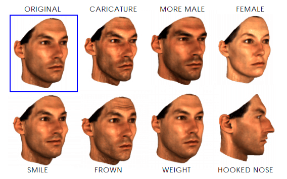
However, this approach requires a human to label a set of images and manually assign labels \(\mu_i\), which describe the markedness of specific attributes. We iterate through all the faces and the parameter \(\mu_i\) will be like the weight parameter. For example, for binary attributes, such as gender, we assign constant values to this parameter. We want to calculate features for all females in our dataset, we set the \(\mu_i = 1\) and all males to \(\mu_i = 0\), and this way we will calculate the attribute that corresponds to only female features. This technique is done for geometry and also for texture. Take a look at the formula below.

$$ \triangle S = \sum_{i=1}^{m}\mu_i(S_i-\bar{S}) \quad \textrm{,} \quad \triangle T=\sum_{i=1}^{m} \mu_i(T_i – \bar{T})$$

Matching a Morphable Model to images

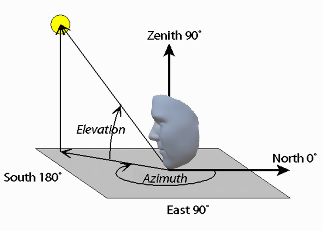
Now we come to an interesting part, how we can match a 3D model to our faces. So, we want to automatically match a 3D model to one or more images. The goal is to find the coefficients of a 3D model for a particular image. Applying PCA to a face we obtain two coefficients, \(\alpha_j\) and \(\beta_j\), which are facial shape and texture. On the other hand, there is a large number of parameters that are needed for further rendering processes. These parameters are defined as \(\overrightarrow{\rho}\), and they include camera position (azimuth and elevation, Figure 10), object scale, image plane rotation, and translation, the intensity of ambient light, and intensity of directed light.

These are a lot of parameters that we haven’t talked about yet, but let us keep them as such and we will understand them later in this post.

Creation of 2D image from 3D model

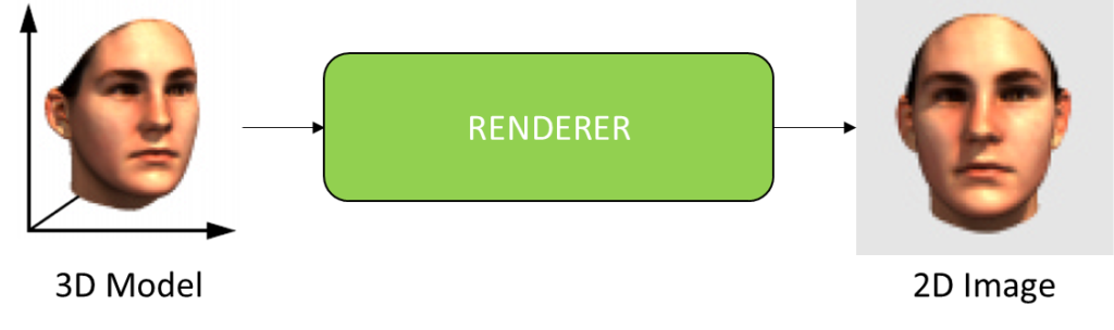
As we have added a new set of parameters to the previous two, we now have that our 3D model consists of \((\overrightarrow{\alpha}, \overrightarrow{\beta}, \overrightarrow{\rho})\). These can help us create a colored image. When we have a 3D model, we can perform rendering, which simply means projecting it into a new dimension, in this case in a 2D space/image, where each vertex will get corresponding lighting, contrast, shadow, etc.

$$ I_{model}(x, y) = (I_{r, mod}(x, y), I_{g, mod}(x, y), I_{b, mod}(x, y))^T$$

We can think of \(I_{model}(x, y)\) as an image that is projected on an image plane. We get this by rendering. Rendering means that there is some algorithm that from a large set of parameters gives us an image. This simply means that we go from a 3D image, that has \((X, Y, Z)\) coordinates of each of the vertices and the corresponding texture for each vertice, to a 2D image (Figure 11).

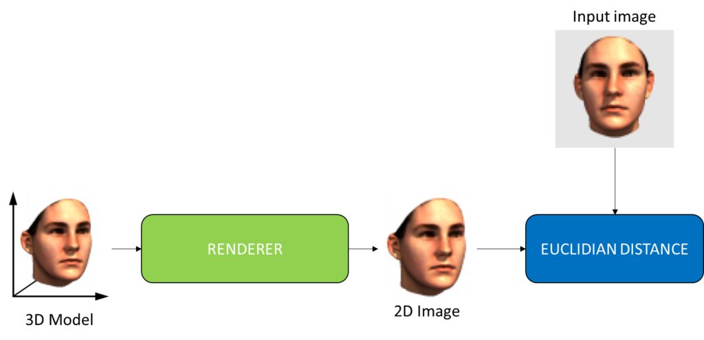
This process can be performed using perspective transformation and the Phong illumination model. But to match a 3D model to an image, take an image and generate a 3D face model of the face on that image, is a different problem. This new 3D model that we want to find should be described as a set of parameters \((\overrightarrow{\alpha}, \overrightarrow{\beta}, \overrightarrow{\rho})\), which we actually want to find. To solve this problem we need to write some objective function and it is written as this:

$$ E_l = \sum\nolimits_{x, y} ||I_{input}(x, y) – I_{model}(x, y)||^2$$

We take the 3D model render it into a 2D image and compare it with the input image using Euclidian distance, or the L2 norm (Figure 12).

Defining a cost function

The scientists call this problem of matching a 3D surface to a given image an ill-posed problem. Along with desired solutions, many non-face-like surfaces lead to the same image. Statistically, it will not make sense, because the parameters will have strange values. So it is essential to impose constraints on the solutions for a set of parameters. Therefore these parameters \((\overrightarrow{\alpha}, \overrightarrow{\beta}, \overrightarrow{\rho})\) need to be restricted in a way that they stay within a boundary, and this is done based on the database, which is done using a regularization term.

Looking at the set of faces, scientists found out that the solutions can further be restricted by a tradeoff between matching quality and prior probabilities. This is done in terms of Bayes decision theory, where we want to find a set of parameters \((\overrightarrow{\alpha}, \overrightarrow{\beta}, \overrightarrow{\rho})\) with maximum posterior probability for a given 2D image. This means that once we have these parameters, we can go from 3D to 2D in a completely deterministic way. However, they say that the input image may not be a perfect face that you have but a noise incorporated into this image.

For the Gaussian noise, they also define a standard deviation \(\sigma_N\), the likelihood to observe \(I_{input}\) is \(p (I_{input}|(\overrightarrow{\alpha}, \overrightarrow{\beta}, \overrightarrow{\rho})) \sim exp[\frac{1}{2\sigma^{2}_{N}} \dot{} E_I]\). Using a method called Maximum likelihood they define the following cost function that needs to be minimized:

$$ E = \frac{1}{2\sigma^{2}_{N}}E_I + \sum_{j=1}^{m-1}\frac{\alpha^2_j}{\sigma^2_{S,j}}+ \sum_{j=1}^{m-1}\frac{\beta^2_j}{\sigma^2_{T,j}} + \sum_{j}{}\frac{(\rho_j – \bar{\rho_j})^2}{\sigma^2_{\rho,j}}$$

Where \(E_I\) represents the Euclidian distance we described before, and in which the parameters are also hidden. These parameters can be seen as regularization parameters, which means that we really want to get values that match the values we get from the PCA model.

Optimizing the cost function

Next, the easiest way to evaluate the color values is in the center of the triangles. They find this center called \(K \), which is the average of the 3D locations \((X_k, Y_k, Z_k)^T\) and textures \((R_k, G_k, B_k)^T\). These triangles will give us pixels of interest which will later be mapped using perspective projection to image locations \((\bar{p}_x, k, \bar{p}_y, k)^T\). Now we have these colors and coordinates, but how will this be rendered?

Maybe the face needs to be rendered in a dark space, or a bright space. So we need to take all the rendering parameters into account and then obtain certain variants of the color. To do this, we have surface normals \(n_k\) of each of the triangles, and we know whether this normal is pointing at the light or in some other direction. So, according to Phong Illumination the color components \((I_{r, model},I_{g, model},I_{b, model})\) take the form:

$$ I_{r, model, k} = (i_{r, amb} + i_{r, dir} * (n_kl))\bar{R}_k + i_{r, dir}s*(r_k v_k)^v$$

where \(amb\) refers to the parameters of the ambient lighting, \(dir\) refers to the direct light, and \(n_k\) to the normal that we just mentioned. So the equation above is displayed for the red color channel, this is done for the other channels as well. But, if we assume that the shadow is cast on the center of the triangle, the equation is reduced to:

$$ I_{r, model, k} = i_{r, amb}R_k$$

This all means, that for the image we will not calculate each pixel, but rather take the center of the triangles and project them to the image. So we can modify our L2 norm the following way.

$$ E_l \approx \sum_{k=1}^{n_t} a_k * ||I_{input}(\bar{p}_x,k,\bar{p}_y,k) – I_{model, k}||^2 $$

In the formula, we are comparing the centers of each triangle in the modeled image and the input image. The variable \(a_k\) is the image area covered by triangle \(k\), but if the triangle is occluded then \(a_k = 0\). This means that if one triangle does not match in color but is large, its area is large, it will influence more this model.

Instead of picking all the triangles, there are many of them, we pick only 40 of these triangles and calculate the distance based on them. How do we pick 40 triangles? Based on the area of the triangle we pick the triangles with the biggest areas. Partial derivatives of the parameters are calculated in an analytical way, depending on the reduced cost function \(E\). This is done in the following way: \(a_j \to a_j – \lambda_j * \frac{\partial E}{\partial \alpha_j}\) and similarly for \(\beta_j\) and \(\rho_j\).

The derivatives of textures and shapes give us derivatives of 2D locations \((\bar{p}_x,k,\bar{p}_y,k)^T\), surface normals \(n_k\), vectors \(v_k\), and \(r_k\), and \(I_{model}\) using the chain rule. From the reduced euclidian distance formula partial derivatives \(\frac{\partial E_K}{\partial \alpha_j}\), \(\frac{\partial E_K}{\partial \beta_j}\) and \(\frac{\partial E_K}{\partial \rho_j}\) can be obtained.

Summary

That is it for this post. In this article, we covered a very interesting topic. We introduced a well-known technique for modeling textured 3D faces. We explained that by converting a set of 3D face models’ shapes and textures into a vector space representation, we will be able to create a morphable face model. Then, we learned that we can create a linear combination of the models, and generate new faces and facial expressions.

References

[1] Zhang, Xiaozheng & Zhao, Sanqiang & Gao, Yongsheng. (2008). Lighting Analysis and Texture Modification of 3D Human Face Scans. 402 – 407. 10.1109/DICTA.2007.4426825.

[2] Blanz, Volker, and Thomas Vetter. “A morphable model for the synthesis of 3D faces.” Proceedings of the 26th annual conference on Computer graphics and interactive techniques. 1999.

[3] WHAT ARE THE “AZIMUTH AND ELEVATION” OF A SATELLITE? https://www.celestis.com/resources/faq/what-are-the-azimuth-and-elevation-of-a-satellite/