#003 Advanced Computer Vision – Multi-Task Cascaded Convolutional Networks

Highlights: Face detection and alignment are correlated problems. Change in various poses, illuminations, and occlusions in unrestrained environments can make these problems even more challenging.

In this tutorial, we will study how deep learning approaches can be great performing solutions for these two problems. We will study a deep cascaded multi-task framework proposed by Kaipeng Zhang [1] et al. that predicts face and landmark location in a coarse-to-fine manner. So let’s get started!

Tutorial Overview:

1. Introduction To Face Detection & Alignment
   • Significance
   • Use Of CNN
2. The Zhang Et Al. Approach
   • Basic Framework
   • CNN Architecture
   • Training The CNNs
3. Multi-Source Training
4. Online Hard Sample Mining
   

1. Introduction To Face Detection & Alignment

Significance

Recognizing faces and expressions involves crucial face detection and alignment solutions. But with facial variations, occlusions, pose differences, and lighting challenges, the task at hand becomes even more difficult.

To make these tasks more efficient, Viola and Jones trained cascaded classifiers using Haar-Like features and AdaBoost. Even though this Cascade Face Detector achieved good performance, it was found that it may degrade significantly when faced with larger visual variations of human faces. Then, there are Deformable Part Models (DPM) which are also used for face detection. These models achieve remarkable performance as well, however, they are computationally expensive.

Use Of CNN

More recently, Convolutional Neural Networks (CNNs) have gained popularity in solving Computer Vision tasks like image classification and face recognition. The deep CNN for facial attribute recognition, trained by Yang et al. and the cascaded CNNs for face detection by Li et al. are some of the famous examples.

In the case of face alignment, the popular approaches include Regression-based methods and Template-fitting methods. The proposal to use facial attribute recognition as an auxiliary task in order to elevate the performance of face alignment, by Zhang et al., is a popular example in this category.

However, the main problem with the methods used for detecting and aligning faces is that they ignore that the two tasks are correlated. There have been attempts by Chen et al. and Zhang et al. to jointly solve the two tasks but they are not entirely efficient.

An important aspect of effective face detection and alignment is the training process and the detector used to mine hard samples. Traditional methods were performed offline. However, for a truly adapting training process, the hard sample mining method must be entirely done online. This is critical for strengthening the power of the detector during the training process.

In this blog post, we will learn about a new framework proposed by Zhang et al., which uses unified cascaded CNNs to solve face detection and alignment together. We will also see how the researchers designed a lightweight CNN architecture to achieve real-time performance. And then, we will study how an effective method was proposed to conduct online hard sample mining.

Let’s start by understanding the basic framework of the model.

2. The Zhang Et Al. Approach

The proposed method by Zhang et al. involves three-stage multi-task deep convolution networks, as can be seen in the image below.

Let’s understand the three stages of this proposed framework in detail.

Basic Framework

The very first step in the pipeline of events is to receive an input image.

Once the image is received, it is resized to different scales and an image pyramid is constructed. This image pyramid becomes the input to the first stage of the proposed cascaded framework.

Stage-1: Essentially, in the first stage, the candidate windows are rapidly produced using a shallow CNN. This fully convolutional network, known as the Proposal Network (P-Net) is used to obtain the candidate windows and their respective bounding box regression vectors. These estimated vectors are then used to calibrate the candidates. A Non-Maximum Suppression (NMS) is finally employed so that candidates, which are highly overlapped, can be merged.

Stage-2: After the first stage, each of the candidates is fed to a Refine Network (R-Net). This is a more complex CNN than what was used in Stage-1 and it further rejects a large number of false candidates. This network also employs bounding box regression vectors to perform calibration and utilizes the NMS for candidate merge.

Stage-3: Finally, the result of Stage-2 is further refined and the network outputs the positions of five facial landmarks. The CNN utilized in this stage is even more powerful than the previous ones and is known as the Output Network (O-Net).

Now that we have gained a basic understanding of the overall pipeline of the proposed approach, let’s see what the architecture is like for each of the CNNs described above.

CNN Architectures

As we learned that there are three types of CNNs used in the approach proposed by Zhang et al., namely, P-Net, R-Net, and O-Net. We can see their respective pictorial representations in the image below.

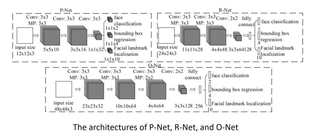
While working with these CNNs, the researchers noted that the performances of each of these networks might be limited due to the lack of diversity of weights in some of the filters. This may restrict the production of discriminative descriptors. In addition, face detection is a challenging binary classification task that involves fewer filters but more discrimination, unlike other multi-class objection detection and classification tasks.

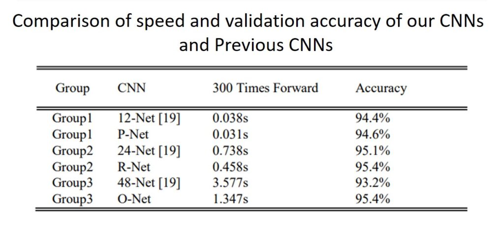
Therefore, in order to reduce the computational expense, the number of filters was reduced and the \(3\times3 \) filter was used instead of a \(5\times5 \) filter. Also, the depth was increased so that better performance is achieved with lesser runtime. Have a look at the result below.

Let’s move ahead and learn how each of these CNN detectors is trained.

Training The CNNs

The CNN detectors used by Zhang et al. in their proposed face detection and alignment method were trained by the researchers using three main techniques.

1. Face Classification: This is essentially a two-class classification problem that indicates whether a given sample is a ‘Face’ or a ‘Non-Face’. So, for a given sample \(x_{i} \), the cross-entropy loss can be calculated as follows.
   
   $$ L_{l}^{\text {det }}=-\left(y_{i}^{\text {det }} \log \left(p_{i}\right)+\left(1-y_{l}^{\text {det }}\right)\left(1-\log \left(p_{i}\right)\right)\right) $$
   
   In the expression above, \(p_{i} \) represents the probability of a sample being a face. The ground-truth label is denoted by \(y_{l}^{\text {det }} \in{0,1} \).
   
   
2. Bounding Box Regression: The learning objective, here, is seen as a regression problem that predicts the offset between each candidate window and its nearest ground truth, i.e., the bounding boxes’ left top, height, and width. For a given sample \(x_{i} \), the Euclidean loss can be calculated as follows.
   
   $$ L_{i}^{b o x}=\left\|\hat{y}_{i}^{b o x}-y_{i}^{b o x}\right\|_{2}^{2} $$
   
   Here, the regression target given by the network is represented as \(\hat{y}_{i}^{\text {box }} \) and the ground-truth coordinate is denoted by \(y_{i}^{\text {box }} \). Since there are four coordinates – left, top, height, and width, it could be said that \(y_{i}^{b o x} \in \mathbb{R}^{4} \).
   
   
3. Facial Landmark Localization: This task is computed similar to the Bounding Box Regression task because even this can be formulated as a regression problem and the Euclidean loss can be minimized as written below.
   
   $$ L_{i}^{\text {landmark }}=\left\|\hat{y}_{i}^{\text {landmark }}-y_{i}^{\text {landmark }}\right\|_{2}^{2} $$
   
   In the expression above, the coordinate of the facial landmark given by the network is represented as \(\hat{y}_{i}^{\text {landmark }} \), and the ground-truth coordinate is denoted by \(y_{i}^{\text {landmark }} \). Here, we work with five facial landmarks – left eye, right eye, nose, left mouth corner and right mouth corner. Thus, it could be said that \(y_{l}^{\text {landmark }} \in \mathbb{R}^{10} \).
   

Let us move ahead and learn about how CNNs performing individual tasks can be trained from more than one source.

3. Multi-Source Training

Each CNN is employed to solve different tasks. Due to this, there are various kinds of training images in the learning process such as Face, Non-Face, and Partially Aligned Face. The researchers decided to skip using the loss functions in two of the three CNNs discussed above.

So, for the sample of the background region, only \(L_{l}^{\text {det }} \) was computed and other losses were set to 0. As a result, the overall learning target could now be written as:

$$ \min \sum_{i=1}^{N} \sum_{j \in{\text { det }, \text { box }, \text { landmark }}} \alpha_{j} \beta_{i}^{j} L_{i}^{j} $$

Here, \(N \) is the number of training samples, \(\alpha_{j} \) denotes the task importance and \(\beta_{i}^{j} \in{0,1} \) is the sample type indicator.

For P-Net and R-Net: \(\alpha_{\text {det }}=1 \), \(\alpha_{\text {box }}=0.5 \), \(\alpha_{\text {landmark }}= 0.5 \)

For O-Net: \(\alpha_{\text {det }}=1 \), \(\alpha_{\text {box }}= 0.5 \), \(\alpha_{\text {landmark }}=1 \)

The above values help in increasing the accuracy of facial landmarks localization.

Clearly now, the overall process of training CNNs using this method becomes a stochastic gradient descent problem. Moving on, let’s see how hard samples were mined traditionally and how conventional online mining is better suited for an effective model.

4. Online Hard Sample Mining

In order to adapt to the training process in the face classification task effectively, the researchers conducted online hard sample mining instead of the traditional one.

What this means is that they sorted the loss computed in the forward propagation phase and chose the top 70% as hard samples and ignored the easy samples which weren’t helpful in strengthening the detector while training.

Next, for each of these hard samples, the gradient was computed in the backward propagation phase. And, finally, experiments were conducted which proved that this strategy yielded better performance without manual sample selection.

Now, let’s see how we can use MTCNN to extract faces and features from images and videos in Python.

5. MTCNN in Python

First, we need to install the MTCNN library. We can easily do that because the MTCNN library is available as a pip package. So, we are going to use the following command.

pip install mtcnn

Next, let’s import the necessary libraries.

import mtcnn

import matplotlib.pyplot as plt

from google.colab.patches import cv2_imshowCode language: JavaScript (javascript)

To check the installation we can just print the MTCNN version.

# print version
print(mtcnn.__version__)Code language: PHP (php)

Output:

0.1.0

Now when we know that our installation is successfully executed, we are ready to proceed with our code. In order to detect faces and keypoints we will define a function draw_facebox(). We will use this function to draw the rectangle around the face and to draw circles at keypoints locations.

# draw an image with detected objects
def draw_facebox(filename, result_list):
  data = plt.imread(filename)
  plt.imshow(data)
  ax = plt.gca()
  for result in result_list:
    x, y, width, height = result['box']
    rect = plt.Rectangle((x, y), width, height,fill=False, color='green',lw=4)
    ax.add_patch(rect)
    for key, value in result['keypoints'].items():
      dot = plt.Circle(value, radius=2, color='red')
      ax.add_patch(dot)
    plt.show()Code language: PHP (php)

Next, we will load the image. Then, we will call the mtcnn.MTCNN() function and create an object called faces where we are going to store detected faces and keypoints. The function mtcnn.MTCNN() returns a list of coordinates, of a rectangle where the MTCNN algorithm detected faces and keypoints.

Finally, we will use the function draw_facebox() to draw rectangles and circles. The first parameter for this function is our image and a second parameter is an object faces where all faces and keypoints are stored.

filename = 'Picture1.jpg' 

pixels = plt.imread(filename)
detector = mtcnn.MTCNN()
faces = detector.detect_faces(pixels)
draw_facebox(filename, faces)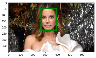Code language: JavaScript (javascript)

To better understand how MTCNN algorithm works, let’s print the object faces.

print(faces)Code language: PHP (php)

Output:

[{‘box’: [264, 45, 125, 177], ‘confidence’: 0.9989251494407654,

‘keypoints’: {‘left_eye’: (289, 120), ‘right_eye’: (351, 117), ‘nose’: (318, 160), ‘mouth_left’: (295, 184), ‘mouth_right’: (349, 183)}}]

As you can see, the “box” value returns the location of the whole face, followed by a “confidence” level, where “keypoints” value returns coordinates of five points: left eye, right eye, nose, left corner of a mouth, and right corner of a mouth.

Now, let’s test this function on another image with no faces.

filename = 'Picture2.jpg' 

pixels = plt.imread(filename)
detector = mtcnn.MTCNN()
faces = detector.detect_faces(pixels)
draw_facebox(filename, faces)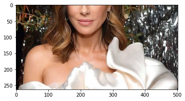Code language: JavaScript (javascript)

As you can see the MTCNN algorithm did not detect anything on this image.

Well, that’s it! We have reached the end of yet another interesting topic of study. Face detection and alignment may seem like two different tasks if you look at them traditionally. But, modern research is able to provide answers on solving these two tasks jointly and effectively. We studied one of the defining researches in this area and learned how Zhang et al. proposed a high-achieving framework for detecting and aligning faces, together.

Face Detection And Alignment

• Face detection and alignment are interrelated
• Variations in the face, pose and illumination can make these tasks more challenging
• Traditional CNN methods didn’t correlate the two tasks and mined hard samples manually
• The approach proposed by Zhang et al. employs three-stage multi-task deep CNNs
• Three different CNNs were used in this approach, viz., P-Net, R-Net, and O-Net
• Multi-source training was performed since each CNN is performing a different task
• Online hard sample mining yields better performance than manual sample selection
  
  

Summary

So folks, how was today’s tutorial? Did you have fun learning about face detection and alignment? If you’d like to understand something deeper or share feedback or connect with like-minded Machine Learning enthusiasts, drop a comment below. Till then, stay safe, stay healthy, and keep multi-tasking! See you. 🙂

References:

[1] Zhang, Kaipeng, et al. “Joint face detection and alignment using multitask cascaded convolutional networks.” IEEE Signal Processing Letters 23.10 (2016): 1499-1503.